

Signal Processing of Random Physiological Signals - Charles S. Lessard
.pdfFAST FOURIER TRANSFORM 151
Symmetric property of twiddle factor implies:
WNk = WNk+ N2 |
= W8k = −W8k+4, which gives |
W80 = −W84 |
W82 = −W86 |
W81 = −W85 |
W83 = −W87 |
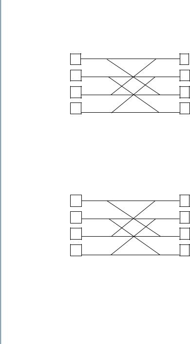
13.6.1 Butterfly First-Stage Calculations
x(0)
x(4)
H1
H2
H1 = x(0) + W80 x(4) = (1 + j × 0) + (1 + j × 0)(−1 + j × 0) = 0 + j × 0 H2 = x(0) − W80 x(4) = (1 + j × 0) − (1 + j × 0)(−1 + j × 0) = 2 + j × 0
x(2)
x(6)
H3
H4
H3 = x(2) + W80 x(6) = (0 + j × 0) + (1 + j × 0)(0 + j × 0) = 0 + j × 0 H4 = x(2) − W80 x(6) = (0 + j × 0) − (1 + j × 0)(0 + j × 0) = 0 + j × 0
x(1)
x(5)
H5
H6
H5 = x(1) + W80x(5) = (0.707 + j × 0) + (1 + j × 0)(−0.707 + j × 0) = 0 + j × 0 H6 = x(1) − W80x(5) = (0.707 + j × 0) − (1 + j × 0)(−0.707 + j × 0)
= 1.414 + j × 0
x(3)
x(7)
H7
H8
H7 |
= x(3) + W80x(7) |
= (−0.707 + j × 0) |
+ (1 + j × 0)(0.707 |
+ j × 0) = 0 + j × 0 |
H8 |
= x(3) − W80x(7) |
= (−0.707 + j × 0) |
− (1 + j × 0)(0.707 |
+ j × 0) |
|
= − 1.414 + j |
× 0 |
|
|
152 SIGNAL PROCESSING OF RANDOM PHYSIOLOGICAL SIGNALS
It should be noted that only W80 → W80 needs to be calculated for the first stage.
13.6.2 Second-Stage Calculations
H1
H2
G1
G2
|
|
H3 |
G3 |
|
|
|
H4 |
G4 |
|
G 1 |
= H1 |
+ W80 H3 |
= (0 + j × 0) + (1 + j × 0)(0 + j × 0) = 0 + j × 0 |
|
G 2 |
= H2 |
+ W80 H4 |
= (2 + j × 0) + (1 + j × 0)(0 + j × 0) = 2 + j × 0 |
|
G 3 |
= H1 |
− W80 H3 |
= (0 + j × 0) − (1 + j × 0)(0 + j × 0) = 0 + j × 0 |
|
G 4 |
= H2 |
− W80 H4 |
= (2 + j × 0) − (1 + j × 0)(0 + j × 0) = 2 + j × 0 |
|
|
|
H5 |
G5 |
|
|
|
H6 |
G6 |
|
|
|
H7 |
G7 |
|
|
|
H8 |
G8 |
|
G 5 = H5 + W80 H7 = (0 + j × 0) + (1 + j × 0)(0 + j × 0) = 0 + j × 0 G 6 = H6 + W80 H8 = (1.414 + j × 0) + (1 + j × 0)(−1.414 + j × 0)
= 1.414 − j × 1.414
G 7 = H5 − W80 H7 = (0 + j × 0) − (1 + j × 0)(0 + j × 0) = 0 + j × 0 G 8 = H6 − W80 H8 = (1.414 + j × 0) − (1 + j × 0)(−1.414 + j × 0)
= 1.414 + j × 1.414

FAST FOURIER TRANSFORM 153
13.6.3 Third-Stage Calculations
G1
G2
G3
G4
G5
G6
G7
G8
X(0)
X(1)
X(2)
X(3)
X(4)
X(5)
X(6)
X(7)
X(0) = G 1 |
+ W80G 5 = (0 + j × 0) + (1 + j × 0)(0 + j × 0) = 0 + j × 0 |
|||||
X(1) = G 2 |
+ W81G 6 = (2 + j × 0) |
+ (0.707 + j × 0.707)(1.414 − j × 1.414) |
||||
|
= 4 + j × 0 |
|
|
|
|
|
X(2) = G 3 |
+ W82G 7 = (0 + j × 0) |
+ (0 + j × 1)(0 + j × 0) = 0 + j × 0 |
||||
X(3) = G 4 |
+ W83G 8 |
= (2 + j × 0) |
+ (−0.707 + j × 0.707)(1.414 + j × 1.414) |
|||
|
= 0 + j × 0 |
|
|
|
|
|
X(4) |
= G 1 |
− W80G 5 = (0 + j × 0) − (1 + j × 0)(0 + j × 0) = 0 + j × 0 |
||||
X(5) |
= G 2 |
− W81G 6 |
= (2 + j × 0) |
− (0.707 + j × 0.707)(1.414 − j × 1.414) |
||
|
= 0 + j × 0 |
|
|
|
|
|
X(6) |
= G 3 |
− W82G 7 |
= (0 + j × 0) |
− (0 + j × 1)(0 + j × 0) = 0 + j × 0 |
||
X(7) |
= G 4 |
− W83G 8 |
= (2 + j × 0) |
− (−0.707 + j × 0.707)(1.414 + j × 1.414) |
||
|
= 4 + j × 0 |
|
|
|
|
|
Each of the eight samples for x(nt) is given by |
||||||
|
|
x(0) |
= 1 + j × 0 |
|
x(4) = −1 + j × 0 |
|
|
|
x(1) |
= 0.707 + j × 0 |
x(5) = −0.707 + j × 0 |
||
|
|
x(2) |
= 0 + j × 0 |
|
x(6) = 0 + j × 0 |
|
|
|
x(3) |
= −0.707 + j × 0 |
x(7) = 0.707 + j × 0 |
||

154SIGNAL PROCESSING OF RANDOM PHYSIOLOGICAL SIGNALS
13.6.4The DFT by Directed Method
In comparison, the direct calculation would be as follows:
N−1 |
|
j 2π |
x (k) = x (n) × (WN )nk |
k = 0, 1, . . . N − 1 WN = e − |
|
N |
||
n=0 |
|
|
X(0) = x(0)W 0 + x(1)W 0 + x(2)W 0 + x(3)W 0 + x(4)W 0 + x(5)W 0 + x(6)W 0 + x(7)W 0
=(1+ j × 0)+(0.707 + j × 0)+(0 + j × 0)+(−0.707 + j × 0)+(−1 + j × 0)
+ (−0.707 + j × 0) + (0 + j × 0) + (0.707 + j × 0) = 0 + j × 0
X(1) = x(0)W 0 + x(1)W 1 + x(2)W 2 + x(3)W 3 + x(4)W 4 + x(5)W 5 + x(6)W 6
+x(7)W 7 = (1 + j × 0) + (.5 + j × 0) + (0 + j × 0) + (0.5 + j × 0)
+(1 + j × 0) + (0.5 + j × 0) + (0 + j × 0) + (0.5 + j × 0) = 4 + j × 0
X(2) = x(0)W 0 + x(1)W 2 + x(2)W 4 + x(3)W 6 + x(4)W 8 + x(5)W 10 + x(6)W 12
+x(7)W 14 = (1 + j × 0) + (0 + j × 0) + (0 + j × 0) + (0 + j × 0)
+(−1 + j × 0) + (0 + j × 0) + (0 + j × 0) + (0 + j × 0) = 0 + j × 0
X(3) = x(0)W 0 + x(1)W 3 + x(2)W 6 + x(3)W 9 + x(4)W 12 + x(5)W 15 + x(6)W 18
+x(7)W 21 = (1 + j × 0) + (−0.5 + j × 0) + (0 + j × 0) + (−0.5 + j × 0)
+(1 + j × 0) + (−0.5 + j × 0) + (0 + j × 0) + (−0.5 + j × 0) = 0 + j × 0
X(4) = x(0)W 0 + x(1)W 4 + x(2)W 8 + x(3)W 12 + x(4)W 16 + x(5)W 20 + x(6)W 24
+x(7)W 28 = (1 + j × 0)+ (−0.707+ j × 0) + (0 + j × 0)+ (0.707 + j × 0)
+(−1 + j × 0) + (0.707 + j × 0) + (0 + j × 0) + (−0.707 + j × 0) = 0
+j × 0
X(5) = x(0)W 0 + x(1)W 5 + x(2)W 10 + x(3)W 15 + x(4)W 20 + x(5)W 25 + x(6)W 30
+x(7)W 35 = (1 + j × 0) + (−0.5 + j × 0) + (0 + j × 0) + (−0.5 + j × 0)
+(1 + j × 0) + (−0.5 + j × 0) + (0 + j × 0) + (−0.5 + j × 0) = 0 + j × 0

FAST FOURIER TRANSFORM 155
X(6) = x(0)W 0 + x(1)W 6 + x(2)W 12 + x(3)W 18 + x(4)W 24 + x(5)W 30 + x(6)W 36
+x(7)W 42 = (1 + j × 0) + (0 + j × 0) + (0 + j × 0) + (0 + j × 0)
+(−1 + j × 0) + (0 + j × 0) + (0 + j × 0) + (0 + j × 0) = 0 + j × 0
X(7) = x(0)W 0 + x(1)W 7 + x(2)W 14 + x(3)W 21 + x(4)W 28 + x(5)W 35 + x(6)W 42
+x(7)W 49 = (1 + j × 0) + (0.5 + j × 0) + (0 + j × 0) + (0.5 + j × 0)
+(1 + j × 0) + (0.5 + j × 0) + (0 + j × 0) + (0.5 + j × 0) = 0 + j × 0
13.6.5The DFT by FFT Method
|
N−1 |
|
7 |
|
|
|
|
− |
j 2π |
|
|
|
|
|
|
|
X (k) = x (n) WNnk = |
x (n) W8nk ; |
W8 = e |
8 |
; k = 0, 1, . . . 7 |
|
|
||||||||||
|
n=0 |
|
n=0 |
|
|
|
|
|
|
|
|
|
|
|
|
|
|
3 |
nk |
k |
3 |
|
nk |
|
|
|
|
|
− j 2π |
|
|
|
|
= |
|
|
|
; |
|
W4 = e |
|
|
|
|
|
|||||
x (2n) W4 |
+ W8 |
x (2n + 1) W4 |
|
|
4 ; k = 0, 1, . . . 3 |
|||||||||||
|
n=0 |
|
|
n=0 |
|
|
|
|
|
|
|
|
|
|
|
|
|
1 |
|
|
1 |
|
|
|
|
|
|
|
|
|
|
|
|
= x (4n) W2nk + W4k |
x (4n + 2) W2nk |
|
|
|
|
|
|
|
|
|
|
|||||
|
n=0 |
1 |
|
n=0 |
|
1 |
|
|
|
|
|
|
|
|
|
|
|
k |
|
nk |
k |
|
|
|
nk |
|
|
|
− j 2π |
|
|
||
|
|
|
x (4n + |
|
|
|
|
; |
k = 0, 1 |
|||||||
|
+W8 |
x (4n + 1) W2 |
+ W4 |
3) W2 |
; W2 = e 2 |
|||||||||||
|
|
n=0 |
|
|
|
n=0 |
|
|
|
|
|
|
|
|
|
|
Periodicity property of Twiddle factor used in the FFT implies:
WNK = WNN+K or W8K = WN8+K
Therefore, one needs to calculate the twiddle factor for W80 → W87.
13.7 SUMMARY
In summary, the usefulness of the FFT is the same as the DFT in Power Spectral Analysis or Filter Simulation on digital computers; however, the FFT is fast and requires fewer computations than the DFT. Decimation-in-time is the operation of separating the input data series, x(n) into two N/2 length sequences of even-numbered points and of odd-numbered points, which can be done as long as the length is an even number, i.e., 2 to any power. Results of the decimation in the FFT are better shown with the “Butterfly”

156 SIGNAL PROCESSING OF RANDOM PHYSIOLOGICAL SIGNALS
Index |
Real (an ) |
Imaginary( j bn ) |
|
0 |
2 |
0 |
DC offset |
1 |
0.5 |
0.95 |
Fundamental ( f0) |
2 |
3 |
2.1 |
2nd Harmonic |
3 |
1.1 |
−6.2 |
3 × f0 |
4 |
0.25 |
−6.7 |
Center fold |
5 |
1.1 |
6.2 |
Conjugate 3 × f0 |
6 |
3 |
−2.1 |
Conjugate 2 × f0 |
7 |
0.5 |
−0.95 |
Conjugate f0 |
FIGURE 13.6: Output values for an eight-sample FFT
signal flow diagram with the number of complex computation Stages as, V = Log2N, since N = 2V . In general, computation of a subsequent stage from the previous butterfly is given by the basic butterfly equations, which reduce the number of complex operations from N 2 for the DFT to N Log2N for the FFT; where N = 2m , and m is a positive integer. The output of the FFT is shown in Fig. 13.6. Note that the first index output is the DC value of the signal. Note that the spectrum folds about the center (index 4) and the output values for indices, 5 through 7, are the conjugate of the output values for indices, 1 through 3.

157
C H A P T E R 1 4
Truncation of the Infinite
Fourier Transform
Problems in the accuracy of the Fourier Transform occur when adherence to the “Dirichlet Conditions” have not been met. Recall the Dirichlet condition requirements on the signal to be transformed as
1.a finite number of discontinuities,
2.a finite number of maxima and minima, and
3.that the signal be absolutely convergent (14.1)
T
f (t) d t < ∞ |
(14.1) |
o
It is impractical to solve an infinite number of transform coefficients; therefore, the engineer must decide how many Fourier coefficients are needed to represent the waveform accurately. How to make a decision on where to truncate the series is a very important part of signal processing.
Truncation means that all terms after the nth term are dropped, resulting in n finite number of terms to represent the signal. However, not including all the coefficients results in an error referred to as the “Truncation error.” The truncation error, εn , is defined as the difference between the original function f (t) and the partial sum, s n (t) of the inverse transformed truncated Fourier terms.
εn = f (t) − s n (t)

158 SIGNAL PROCESSING OF RANDOM PHYSIOLOGICAL SIGNALS
where εn is the truncation error. The partial sum is often expressed as the “mean-squared error” as in (14.2).
|
1 |
T |
|
|
E n = |
[εn (t)]2d t |
(14.2) |
||
T 0 |
To understand truncation of a series, it is important to know what is desirable in
truncation. Since accuracy is one of the most desirable specifications in any application, it would be desirable to attain acceptable accuracy with the least number of terms. Without proof in limits and convergence, let us define convergence as the rate at which the truncated series approaches the value of the original function, f (t). In general, the more rapid the convergence, the fewer terms are required to obtain desired accuracy.
The convergence rate of the Fourier Transform is directly related to the rate of the decrease in the magnitude of the Fourier Coefficients. Recall the Fourier transform
coefficients of a square wave as having the following magnitudes: |
|
|
|
|
||||||||||||||||||||||||
1 |
|
|
1 |
|
|
1 |
|
|
1 |
|
|
|
|
1 |
|
|
||||||||||||
|a3| = |
|
|
; |
|a5| = |
|
|
; |
|a7| = |
|
; |
|a9| = |
|
|
; · · · · ; |
|
|an | = |
|
|
|
|||||||||
3 |
5 |
7 |
9 |
n |
|
|||||||||||||||||||||||
Note that the sequence is the reciprocal of the nth term to the 1st power. |
|
|
|
|||||||||||||||||||||||||
Now let us examine the Fourier transform of the triangular waveform shown in |
||||||||||||||||||||||||||||
Fig. 14.1. |
|
|
|
|
|
|
|
|
|
|
|
|
|
|
|
|
|
|
|
|
|
|
||||||
The Fourier trigonometric series representation is given by (14.3). |
|
|
|
|||||||||||||||||||||||||
|
8V |
1 |
1 |
1 |
|
|
|
|
||||||||||||||||||||
v(t) = |
|
|
|
|
sin ω0t − |
|
|
sin 3ω0t + |
|
|
sin 5ω0t + · · · + |
|
sin nω0t |
(14.3) |
||||||||||||||
π 2 |
32 |
52 |
n2 |
|||||||||||||||||||||||||
Note that the magnitude of the coefficients are the square of the nth term. |
|
|
|
|||||||||||||||||||||||||
1 |
|
|
; |
1 |
|
; |
1 |
|
; |
1 |
; · · · · ; |
|
1 |
|
||||||||||||||
|a3| = |
|
|a5| = |
|
|a7| = |
|
|a9| = |
|
|an | = |
|
|
||||||||||||||||||
32 |
52 |
72 |
92 |
n2 |
|
|||||||||||||||||||||||
It is noted that the Fourier coefficients for a triangular waveform diminish faster (rate of convergence) than the Fourier coefficients for a rectangular waveform. To help in
Odd –T/2 |
|
|
|
–T/4 |
|
|
|
|
|
T/2 |
|
|
|
|
|
|
|
|
|||||
|
|
|
|
|
|
|
|
|
|
|
|
|
|
|
|
|
|
T/4 |
|
|
|
|
|
|
|
|
|
|
|
|
|
||||
|
|
|
|
|
|
|
|
|
|
|
|
FIGURE 14.1: One cycle of a triangular waveform with odd symmetry

TRUNCATION OF THE INFINITE FOURIER TRANSFORM 159
TABLE 14.1: Convergence Table
f (t) |
JUMP-IN IMPULSE-IN DECREASING an |
WAVEFORM |
||
|
|
|
|
|
Square wave |
f (t) |
f (t) |
1/n |
Discontinuities |
Triangle wave |
f (t) |
f (t) |
1/n2 |
|
Parabolic/ |
f (t) |
f (t) |
1/n3 |
|
sinusoid |
|
|
|
|
· · · |
f k−1(t) |
f k (t) |
1/nk |
Smoother |
− − − |
||||
determining the rate of convergence, a basic expression was formulated called the Law of Convergence.
The law covering the manner in which the Fourier coefficients diminish with increasing “n” is expressed in the number of times a function must be differentiated to produce a jump discontinuity. For the kth derivative, the convergence of the coefficients will be on the order of 1/nk+1. For example, if that derivative is the kth, then the coefficients will converge at the rate shown in (13.4).
|an | ≤ |
M |
and |
|bn | ≤ |
M |
(13.4) |
nk+1 |
nk+1 |
||||
where M is a constant, which is dependent on |
f (t). |
|
|
||
There are two ways to show convergence. Let us look at Table 14.1, the Convergence Table. The left most column of the table denotes the type of waveform with the right most column describing the waveform as going from with discontinuities to smoother. The second and third columns labeled “Jump-in” and “Impulse-in,” respectively. Jump-in means that discontinuity occurs in the function after successive differentiation, where the discontinuities occur in the square-like waveform. Impulse-in means what derivative (successive differentiation) of the function will result in an impulse train. The fourth column gives the general expression for convergence of the coefficients. From the table one may conclude that the smoother the function, the faster the convergence.
160 SIGNAL PROCESSING OF RANDOM PHYSIOLOGICAL SIGNALS
c1 |
Jumps-in f(t) |
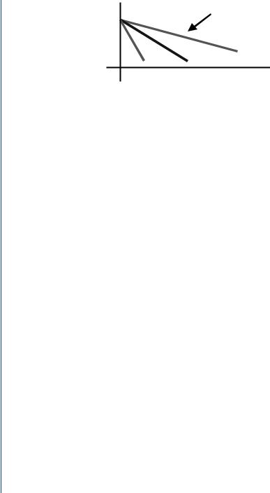
|cn| dB
–6 dB/oct
–12 dB/oct
–18 dB/oct
Frequency
FIGURE 14.2: Graphs of convergence rates
Often, the rates of decrease in the Fourier coefficients with the number of terms, n, are expressed in the logarithmic terms of decibels per octave by expressing the absolute magnitude of the Fourier coefficients, |cn | in decibels and plotting the coefficients against frequency as shown in Fig. 14.2.
14.1 PRACTICAL APPLICATIONS
So how realistic are discontinuities in the real world, specifically physiological signals in clinical and biomedical engineering? Unfortunately, discontinuities in medicine are real. Discontinuities in the human and animal physiological waveforms may be found in the following signals:
1.Electroencephalograms (EEG); Seizure waveforms
2.Spike waveforms in EEG and Electromyogram (EMG)
3.Saccadic movements in the Electro-occulograms (EOG)
It is important to understand what problems discontinuities present in signal processing. It is well known that as more coefficients are added to the waveform approximation, the accuracy improves everywhere except in the immediate vicinity of a discontinuity. Even in the “Limit” as n → ∞, the discrepancy (error) at the point of discontinuity becomes approximately 9%. This error is known as the Gibbs phenomenon.
One may think of the Gibbs phenomenon as the response to a square pulse, which is the characteristic overshoot and damped oscillatory decay in nonlinear systems (filters). What the discontinuities and the Gibbs phenomenon indicate is that one can