Signal Processing of Random Physiological Signals - Charles S. Lessard
.pdfSPECTRAL ANALYSIS 171
1.Filtering: Analog filtering is the first major consideration for the acquisition and processing of data. The engineer must determine the appropriate cutoff frequencies within the signal. Both highand low-frequency cutoff should be determined and appropriate analog filters with sufficient attenuation in the bandstop regions should be employed. The high-pass filter should be used to remove the DC component of the signal and to remove trends. An antialias filter (low-pass filter) should be employed to eliminate “Aliasing” of the data. It is important to use an analog antialias filter prior to sampling of the data; any subsequent digital filtering should be done after sampling.
2.Frequency resolution: Frequency resolution is defined as the smallest unit of frequency in the spectrum. The “Fundamental Frequency” or resolution of the spectrum ( f0 = 1/ T ) is equal to the inverse of time the signal segment (length of time in seconds: T ) that is being analyzed by Spectral Analysis. The segment time is also referred to as the window of observation or analysis. The energy in the spectrum of the signal is identified as harmonics of the fundamental frequency, that is, multiples of the fundamental frequency.
3.Digitizing and the Nyquist criterion: Probably the most important rule to follow in spectral analysis is the Nyquist Criteria in digital sampling of the signal. The sampling rate must be twice the highest frequency of the signal bandwidth (W). Sampling at a frequency lower than the Nyquist frequency causes aliasing of the spectrum, which will then yield an erroneous spectral estimator.
4.Windowing : A “Window” function should be applied prior to obtaining the estimation of the “Spectral Density Function.” Windowing is a process by which the sampled data points are “weighted” in the time domain. The effect is smoothing of the signal at the beginning and end of the record to prevent the occurrence of discontinuities and Gibb’s Phenomenon in the data. Improper windowing produces “Leakage” in the spectrum, which adversely affects estimation of the Spectral Density Function. There are numerous window functions that can be applied. The problem lies in deciding which window function is the best to apply on the signal being studied.

172SIGNAL PROCESSING OF RANDOM PHYSIOLOGICAL SIGNALS
5.Smoothing: To obtain a fairly good estimator, statisticians would insist on some “Smoothing” function, since the Spectral Density Function or Periodogram is a raw power spectrum estimate that contains high-frequency components. Smoothing is a technique equivalent to low-pass filtering to eliminate the highfrequency components from the spectrum for the final smoothed spectral density estimate.
15.6ADVANCED TOPIC
15.6.1 Brief Description of Autoregressive Spectral Estimation
The concept of smoothing serves as a transition to the Autoregressive (AR) Spectral Estimation Method. The AR Spectral Estimator, also known as the Maximum Entropy Spectral Estimator, is becoming more popular in the engineering community as an accurate estimator of the spectral density function.
To perform the AR Spectral Estimation, it is necessary to do the following procedural steps in order.
1.Fit AR model to data
2.Calculate AR coefficients
3.Enter the AR coefficients into formula for spectrum of AR process.
4.Estimate spectrum of AR process
The AR model of order p is represented by (15.24):
xt = α0 + α1xt−1 + α2xt−2 + · · · · +α p xt− p + zt |
(15.24) |
The order of the model is chosen using Akaike’s Information Criterion (AIC). The coefficients are then calculated from (15.25).
|
N−1 |
|
¯ |
|
¯ |
α |
t=1 |
(xt − x)(xt−1 |
− x) |
||
ˆ k = |
|
N−1 |
¯ |
2 |
(15.25) |
|
|
t=1 |
(xt − x) |
|
|
where x¯ is the mean of the sample record, N is the total number of data points, x(t) is the point at time t, and αˆ k is the approximate estimator of α.

|
|
|
|
|
|
|
|
SPECTRAL ANALYSIS 173 |
|
Another approximation that has often been used is given by (15.26). |
|
||||||||
|
N−1 |
|
2 |
|
N |
2 |
|
||
|
|
|
(xt |
¯ |
= |
¯ |
(15.26) |
||
|
t=1 |
− x) |
|
(xt − x) |
|
||||
|
= |
|
|
t=1 |
|
|
|||
If (15.26) is used then |
|
|
|
|
|
|
|
|
|
αk |
rk , where rk is the kth correlation coefficient. |
|
|||||||
Then the sample correlation coefficients are substituted into the Yule–Walker equations |
|||||||||
(15.27), and the matrix equations are solved for α, the AR coefficients. |
|
||||||||
1 |
r1 |
|
|
|
rp−1 |
α1 |
r1 |
|
|
r2 |
1 r1 |
|
|
rp−2 |
α2 |
r2 |
|
||
− |
− |
− |
− |
|
− |
− |
− |
(15.27) |
|
− |
− |
− |
− |
|
− |
x |
= |
||
|
− |
− |
|
||||||
− |
− |
− |
− |
|
r1 |
− |
− |
|
|
r p−1 |
− − − 1 |
αp |
rp |
|
|||||
Since the Fourier transform is given by (15.28), the autospectral density function |
|||||||||
is estimated by using an AR model of order p as given in (15.29). |
|
||||||||
|
|
|
F (ω) = |
|
+∞ |
γk e − j ωk |
|
(15.28) |
|
|
|
|
k=−∞ |
|
|||||
|
|
|
|
|
|
|
|
||
|
|
σ 2 |
|
p |
|
p |
|
|
|
X(ω) = |
|
1 + |
|
αk e − j ωk + |
αk e j ωk |
(15.29) |
|||
|
π |
|
|||||||
|
|
|
|
k=1 |
k=1 |
|
|
||
where the autocovariance function is γ (k) = σ 2αk . |
|
|
|||||||
It should be noted that the frequency ω varies within the interval (0, π ), where π |
|||||||||
represents the Nyquist Frequency. |
|
|
|
|
|
|
|||
15.6.2 Summary
The cross-spectrum shows the relationship between two waveforms (input and output) in the “Frequency Domain.” The cross-spectrum indicates what frequencies in the output are related to frequencies in the input. The cross-spectrum consists of complex terms, which are termed the coincident spectral density function [Co-spectrum, Cxy( f )] and the

174 SIGNAL PROCESSING OF RANDOM PHYSIOLOGICAL SIGNALS
quadrature spectral density function [Quad-spectrum Qxy(f )]. The cross-spectrum is calculated in the same manner as the autospectrum, via direct Fourier Transform of the two signals or via the cross-correlation function. As with the autospectrum, the “Raw” cross-spectrum must be smoothed, and then normalized to get a good estimation of the cross-spectrum.
15.7SUGGESTED READING
1.Bendat, J., and Piersol, A. G. Random Data Analysis and Measurement Procedures.
New York: Wiley & Sons, Inc., 1986.
2.Chatfield, C. The Analysis of Time Series: An Introduction. London: Chapman & Hall, 1980.
3.Lynn, P. A. An Introduction to the Analysis and Processing of Signals. New York: Wiley & Sons, Inc., 1973.
4.McIntire, D. A. “A Comparative Case Study of Several Spectral Estimators,” In
Applied Time Series Analysis, D. F. Findley, ed., Academic Press, 1978.

175
C H A P T E R 1 6
Window Functions and
Spectral Leakage
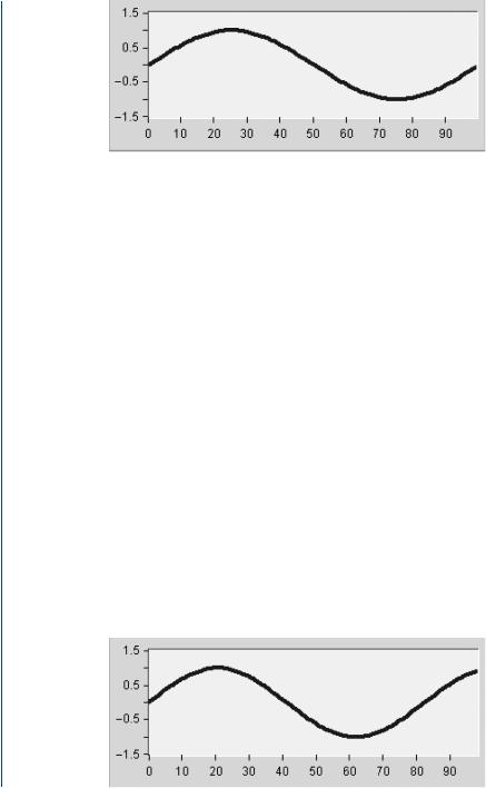
The purpose of window functions is to minimize a phenomenon called “Spectral Leakage,” which is the result of selecting a finite time interval and a nonorthogonal trigonometric basis function over the interval of analysis. Only frequencies that coincide with the basis function will project on a single basis vector, such as shown in Fig. 16.1. Signals, which include frequencies not on the basis set, will not be periodic in the observing interval (often referred to as the “Observation or Observing Window”). The periodic extension of a signal with a period that is not equal to the fundamental period of the window (as in Fig. 16.2) will produce discontinuities at the boundaries of the observing interval. It is these discontinuities that cause the frequency leakage of the signal across the spectrum.
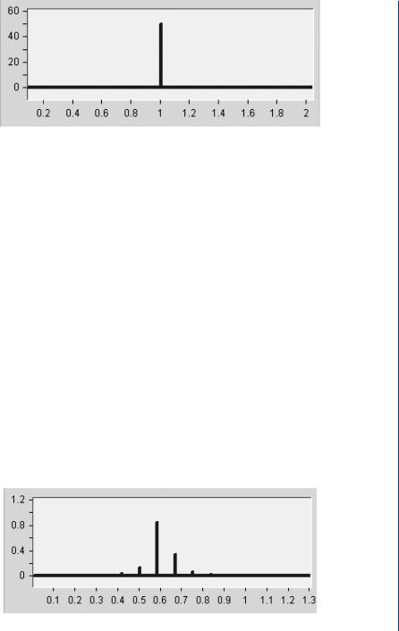
The sine function in Fig. 16.2 does not fit perfectly in the window, since its value at the beginning is not the same as the value at the end of the observation interval [4]. Since the window is supposed to contain a periodic function, one should note that in the next cycle, the value must go from 1 to 0 at the same instant of time. Hence, the discontinuity at the edge of the window will result in the spectral power of a specific frequency leaking out of the main lobe or specific spectral bandwidth to adjacent spectral side lobes. Leakage into the side lobes may occur in either side (direction) of the main lobe. The decrease of power from the main lobe adds to the power in the sideband harmonics resulting in an erroneous estimate of power in the sideband harmonics.
176 SIGNAL PROCESSING OF RANDOM PHYSIOLOGICAL SIGNALS
FIGURE 16.1: Sinusoidal waveform. The sine function fits perfectly in the window, since its
value is zero (0) at the beginning and end of the observation interval
Outward leakage can be easily demonstrated by some simple examples. Figure 16.3 shows the Power Spectral Density (PSD) of a sinusoidal with a period that is equal to the observation window length of 1 second. Note that there is only one lobe at 1 Hz.
Figure 16.4 shows the Power Spectral Density (PSD) of a sinusoidal with a period that is not equal to the observation window length of 1 second. Note the main-lobe spectral energy at 0.59 Hz with side lobes at 0.41, 0.50, 0.68, and 0.77 Hz.
In dealing with random physiological data, the possibility of an integral fundamental frequency repetition is very limited; hence, regardless of what sampling window interval is used, leakage will be present in the spectra.
16.1 GENERALITIES ABOUT WINDOWS
The window functions (often called restoring functions) are basically weighting functions applied to the time domain data. Weighting function selection can be made early in the design process because the choices of FFT algorithm and weighting function are independent of each other. Choice of a weighting function to provide the specified
FIGURE 16.2: Discontinuity in sinusoidal waveform
WINDOW FUNCTIONS AND SPECTRAL LEAKAGE 177
FIGURE 16.3: Power spectral density of the trace in Fig. 16.1. Note the main lobe at 1 Hz
without any side lobes
side-lobe level is done without concern for the FFT algorithm that will be used because
1.they work for any length FFT,
2.they work the same for any FFT algorithm, and
3.they do not alter the FFT ability to distinguish two frequencies (resolution).
Window functions, w(t), have the following properties:
1.The w(t) function has to be real, even and nonnegative.
2.The transformed function has to have a main lobe at the origin of the fundamental frequency, and side lobes at both sides to ensure symmetry.
3.If the nth derivative has an “impulse” character, then the peak of the side lobes of the transformed function will decay asymptotically as 6*n dB/octave (least estimate).
FIGURE 16.4: Power spectral density of the trace with discontinuity shown in Fig. 16.2. Note the main lobe of the spectra at 0.59 Hz with side lobes at 0.41, 0.50, 0.68, and 0.77 Hz

178 SIGNAL PROCESSING OF RANDOM PHYSIOLOGICAL SIGNALS
Weighting functions are applied three ways:
1.as a rectangular function, which does not modify the input data,
2.by having all the weighting function coefficients stored in memory, and
3.by computing each coefficient when it is needed.
16.2PERFORMANCE MEASURES
The choice of a weighting function depends on which of the features of the narrowband DFT filters (resolution) are most important to the application. Those features are performance measures of the narrowband filters to analytically compare weighting functions. All these measures, except frequency straddle loss, refer to individual filters. Frequency straddle loss is associated with how filters work together [3].
16.2.1 Highest Side-Lobe Level
Highest side-lobe level (in decibels) is an indication on how large the effect of the side lobes is. Side lobes are a way of describing how a filter responds to signals at frequencies that are not in its main lobe, commonly called its passband. Each FFT filter has several side lobes. With rare exception, the highest side lobe is closest in frequency to the main lobe and is the one that is most likely to cause the passband filter to respond when it should not. For a signal with the maximum point of the main lobe at 0 dB, rectangular window the first side lobe is about −13 dB, relative amplitude. A good leakage suppressor should have its first side lobe much lower than −13 dB. Since side lobes are the result of leakage from the main lobe, then the more side lobes on either side of the main lobe will result in a reduced or lower main lobe magnitude.
16.2.2 Sidelobe Fall-Off Ratio
The peak (amplitude) of side lobes decreases or remains level as they get further away in frequency from the main lobe passband. Side lobe fall-off characteristic is very important since it indicates the rate at which the side lobes are decreasing in magnitude. The

WINDOW FUNCTIONS AND SPECTRAL LEAKAGE 179
rectangular window has a decreasing rate of −6 dB/octave. This means that the next side lobe will be encountered at −13 − 6 = −19 dB. If the side lobes reduce rapidly, then the main lobe of the FFT bands will lose less energy into the sidelobes and the spectra will be less erroneous. Side lobe fall-off performance measure is important for applications with multiple signals that are close in frequency.
16.2.3 Frequency Straddle Loss
Frequency straddle loss is the reduced output of a DFT filter caused by the input signal not being at the filter’s center frequency. Frequencies seldom fall at the center of any filter’s passband. When a frequency is halfway between two filters, the response of the FFT has its lowest amplitude. For a rectangular weighting function, the frequency response halfway between two filters is 4 dB lower than if the frequency were in the center of a filter. Each of the other weighting functions in this chapter has less frequency straddle loss than the rectangular one. This performance measure is important in applications where maximum filter response is needed to detect the frequencies of interest.
16.2.4 Coherent Integration Gain
Coherent integration gain (often referred to as Coherent Gain or Processing Loss) is the ratio of amplitude of the DFT filter output to the amplitude of the input frequency.
N-point FFTs have a coherent gain of N for frequencies at the centers of the filter passbands. Since most weighting function coefficients are less than l, the coherent gain of a weighted FFT is less than N. While weighting functions reduce the coherent integration gain, the combination of this reduction and the improved straddle loss results in an overall signal response improvement halfway between two filters. Like frequency straddle loss, this performance measure is important in applications where maximum filter response is needed to detect the frequencies of interest. To restore the main lobes to their original magnitudes, the FFT coefficients may be multiplied by the inverse of the coherent gain. Window coherent gains are compared as shown in Table 16.1 to the rectangular window gain, which is 1 or 0 dB.