

Signal Processing of Random Physiological Signals - Charles S. Lessard
.pdf31
C H A P T E R 5
Data Acquisition Process
At this point, I would like to change pace and have a discussion of general steps or procedures in data acquisition and processing. The required operations may be divided into 5 primary categories (Fig. 5.1):
1.Data collection,
2.Data recording/transmission,
3.Data preparation,
4.Data qualification, and
5.Data analysis.
5.1DATA COLLECTION
The primary element in data collection is the instrumentation transducer. In general, a transducer is any device which translates power from one form to another. I will not get into this but in general a model might be as shown in Fig. 5.2.
In some cases it is possible to perform all desired data processing directly on the transducer signals in real time. In most cases, this is not practical. After preamplification some initial filtering and postamplification, most signals are recorded on magnetic media. At the present time, some form of storage of the amplified and preconditioned transducer signals are still required.

32 SIGNAL PROCESSING OF RANDOM PHYSIOLOGICAL SIGNALS
In |
Collection |
|
|
Recording |
|
|
Preparation |
|
|
Qualification |
|
|
Analysis |
Out |
|||
|
|
|
|
|
|
|
|
|
|
|
|
|
|||||
|
|
|
|
|
|
|
|
|
|
|
|
|
|
|
|
|
|
FIGURE 5.1: Data acquisition and analysis process
5.2DATA RECORDING/TRANSMISSION
As in the past, magnetic storage systems are the most convenient and desirable type of data storage. In the 1950s through the 1980s, magnetic tape recordings were the only way to store large quantities of data. If a magnetic tape recorder was used, the most widely used method was referred to as “Frequency Modification” (FM) for analog type recordings. Beyond the limitation inherent in the magnetizationreproduce and modulation-demodulation operations, there are a number of miscellaneous problems.
Among the more important of these problems are the errors associated with variations in the speed at which the tape passes over the record and/or reproduce heads. These errors were called “Time Based Errors,” with the most common being “Flutter,” which is the variation of tape velocity from the normal. For the frequency modulation (FM) recording systems, the time based (frequency) is used to represent the amplitude variations of the signal. The error in good high-quality FM recorders is about 0.25%.
Currently, few laboratories still use magnetic tape recordings. The large “Gigabite” disk memories and optical disc with compression techniques are the most common approach to storage of data; however, the data must be in digital format, and thus must be converted from an analog format to a digital format. The advantage of storing the raw data is that different signal-processing methods may be used on the same data and the results compared.
Physical |
Mechanical |
|
|
|
|
|
Electrical |
|
|
|
|
|
Pickoff |
|
|
||||||
quantity |
conversion |
Internal |
Mech Qty. |
conversion |
Elec. |
|||||
|
||||||||||
FIGURE 5.2: General model of a mechanical transducer for data collection, that is, a blood
pressure transducer

DATA ACQUISITION PROCESS 33
5.3DATA PREPARATION
The third step is data preparation of the raw data supplied as voltage time histories of some physical phenomenon. Preparation involves three distinct processes as shown in Fig. 5.3:
1.editing;
2.conversion; and
3.preprocessing.
Data editing refers to preanalysis procedures that are designed to detect and eliminate superfluous and/or degraded data signals. The undesirable parts of the signal may be from acquisition or recording problems that result in excessive noise, movement artifacts, signal dropout, etc. Editing may be through visual inspection of graphic recordings. Normally, experts in the field are invited to perform the inspection and identify those sections of the data that should not be analyzed. Some laboratories use a Hewlett-Packard Real-time spectrum analyzer and preview the data. In short, “Editing is critical in digital processing” and it is best performed by humans, and not by machines.
Data preparation beyond editing usually includes conversions of the physical phenomena into engineering units (calibration) and perhaps digitization. Digitization consists of the two separate and distinct operations in converting from analog to digital signals:
1.Sampling interval, which is the transition from continuous time to discrete time, and
2.Sample quantization: the transition from a continuous changing amplitude to a discrete amplitude representation.
Editing |
|
|
Conversion |
|
|
Preprocessing |
|
|
|
|
|
|
|
|
|
FIGURE 5.3: Data preparation
34 SIGNAL PROCESSING OF RANDOM PHYSIOLOGICAL SIGNALS
Considerations that must be taken into account when digitizing an analog signal will be covered in two chapters: one on Sampling Theory and the second on Analog-to-Digital Conversion.
Prepossessing may include formatting of the digital data (Binary, ASCII, etc., format), filtering to clean up the digital signal, removing any DC offset, obtaining the derivative of the signal, etc. But before getting into digital conversion, let us continue with the data-acquisition process by examining the fourth step of “Random Data Qualification.”
5.4RANDOM DATA QUALIFICATION
Qualification of data is an important and essential part in the statistical analysis of random data. Quantification involves three distinct processes as shown in Fig. 5.4:
1.stationarity,
2.periodicity, and
3.normality.
It is well known in statistics that researchers should not use “parametric statistical methods” unless the data are shown to be “Gaussian Distributed” and “Independent.” If the data are not Gaussian Distributed and Independent, parametric statistics cannot be used and the researcher must then revert to “nonparametric statistical methods.”
Likewise, necessary conditions for Power Spectral Estimation require that the random data be tested for “Stationarity” and “Independence,” which may be tested parametrically by showing the mean and autocorrelation of the random data to be time invariant or by using the nonparametric “RUNS” Test.
After showing the data to be stationary, researchers may examine the data for “Periodicities” (cyclic variations with time). Periodicity may be analyzed via the
|
|
Stationarity |
|
|
Periodicity |
|
|
Normality |
|
|
|
|
|
|
|
|
|
|
|
FIGURE 5.4: Data qualification

DATA ACQUISITION PROCESS 35
Individual |
|
|
Multiple |
|
|
Linear |
|
records |
|
|
records |
|
|
relationships |
|
|
|
|
|
|
|
|
|
FIGURE 5.5: Random data analysis
“Correlation Function” using either Time or Frequency Domain approach. Periodicity may also be analyzed via the “Power Spectral Analysis.” The next step regarding random data may be to examine the distribution of the data (“Is the data Normality distributed?”) or to determine all the basic statistical properties (Moments) of the signal (data).
5.5RANDOM DATA ANALYSIS
The fifth and final step is data analysis of the data supplied as time histories of some physical phenomenon. Data analysis involves three distinct and independent processes dependent on the experimental question and the data set as shown in Fig. 5.5:
1.analysis of individual records,
2.analysis of multiple records, and
3.linear relationships.
If the analysis is to be accomplished on an individual record, that is, one channel of electrocardiogram recording, or one channel of electroencephalogram recording, etc., then either “Autocorrelation Function Analysis” (Time-domain Analysis) or “Autospectral Analysis” (Frequency-domain Analysis) would be preformed on the random data.
If the analysis is to be accomplished on multiple records, that is, more than one channel of recording, then either “Cross-correlation Function Analysis” (Time-domain Analysis) or “Cross-spectral Analysis” (Frequency-domain Analysis) would be preformed on the random data. Multiple Records would be used to determine the “Transfer Functions” of systems when the input stimulus and the output responses are random signals.

36 SIGNAL PROCESSING OF RANDOM PHYSIOLOGICAL SIGNALS
In a relational study, cause and effect, the primary aim would be to determine the relationship of a stimulus to the response. The most popular method for determining linear relationships is to use the least squares regression analysis and to determine the correlation coefficient; however, the least squares regression analysis is difficult to apply in many random data cases. Therefore, an alternative method is to determine the model or transfer function via autoand cross-spectra. In addition, for any model or transfer function, it is necessary to determine how well the transfer functions represent the system process; hence, the investigator must perform a “Coherence Function Analysis” to determine the “Goodness Fit.”

37
C H A P T E R 6
Sampling Theory and
Analog-to-Digital
Conversion
6.1BASIC CONCEPTS
Use of a digital computer for processing an analog signal implies that the signal must be adequately represented in digital format (a sequence of numbers). It is therefore necessary to convert the analog signal into a suitable digital format.
By definition, an analog signal is a continuous physical phenomenon or independent variable that varies with time. Transducers convert physical phenomena to electrical voltages or currents that follow the variations (changes) of the physical phenomena with time. One might say that an electrical signal is an Analog Signal if it is a continuous voltage or current that represents of a physical variable. Analog signals are represented as a deterministic signal, x(t), for use in a differential equation. Or, one may simply state that an analog signal is any signal that is not a digital signal, but then you must define a digital signal. There are three classes of analog signals.
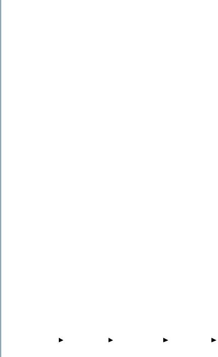
a)Continuous in both time and amplitude (Fig. 6.1).
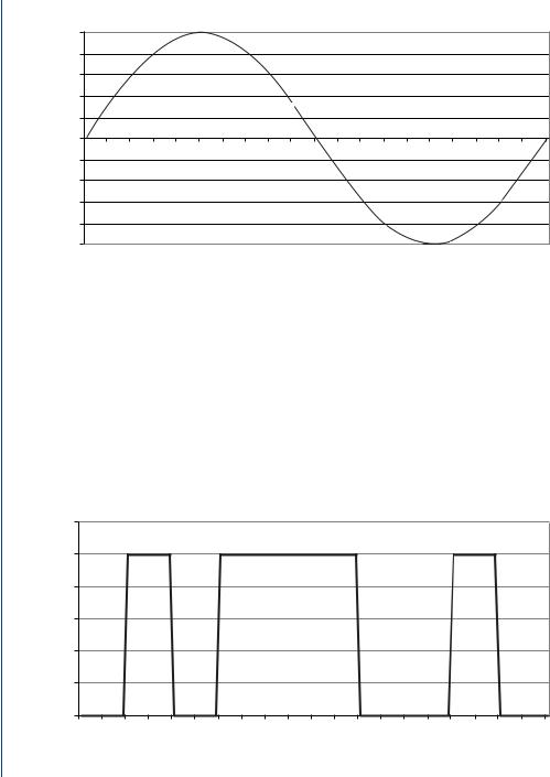
b)Continuous in time (Fig. 6.2) but taking on only discrete amplitude values, that is, analog signals used to approximate digital bit streams in serial communication, which are used primarily for time codes or markers.
38 SIGNAL PROCESSING OF RANDOM PHYSIOLOGICAL SIGNALS
Magnitude
1.0
0.8
0.6
0.4
0.2
0.0 –0.2 0
–0.4
–0.6
–0.8
–1.0
Continuous in time and amplitude
10 |
20 |
30 |
40 |
50 |
60 |
70 |
80 |
90 |
100 |
Time (some unit)
FIGURE 6.1: Analog signal that is continuous in both time and magnitude
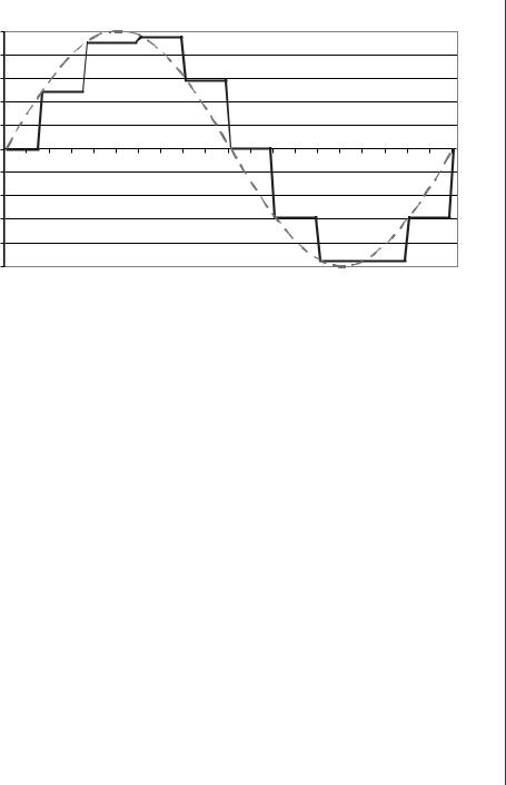
c)Continuous in amplitude (Fig. 6.3) but defined only at discrete points in time, for example, sampled analog signals.
By definition, a digital signal is an ordered sequence of numbers, each of which is represented by a finite sequence of bits; that is, of finite length. It is important to note that a digital signal is defined only at discrete points in time and takes on only one of a
Magnitude
Continuous in time but discrete in magnitude
1.2
1.0
0.8
0.6
0.4
0.2
0.0
0 |
10 |
20 |
30 |
40 |
50 |
60 |
70 |
80 |
90 |
100 |
Time (some unit)
FIGURE 6.2: Analog signal that is continuous in both time and discrete in magnitude
SAMPLING THEORY AND ANALOG-TO-DIGITAL CONVERSION 39
Sampled signal continuous in amplitude but discrete in time
|
1.0 |
|
|
|
|
|
|
|
|
|
|
|
|
0.8 |
|
|
|
|
|
|
|
|
|
|
|
|
0.6 |
|
|
|
|
|
|
|
|
|
|
|
|
0.4 |
|
|
|
|
|
|
|
|
|
|
|
Magnitude |
0.2 |
|
|
|
|
|
|
|
|
|
|
|
0.0 |
|
|
|
|
|
|
|
|
|
|
|
|
–0.2 |
0 |
10 |
20 |
30 |
40 |
50 |
60 |
70 |
80 |
90 |
100 |
|
|
–0.4 |
|
|
|
|
|
|
|
|
|
|
|
|
–0.6 |
|
|
|
|
|
|
|
|
|
|
|
|
–0.8 |
|
|
|
|
|
|
|
|
|
|
|
|
–1.0 |
|
|
|
|
|
|
|
|
|
|
|
Time (some unit)
FIGURE 6.3: An analog signal that has been sampled such that the sampled signal is “continuous in amplitude but defined only at discrete points in time.” The dashed line is the original sinusoidal signal
finite set of discrete values at each of these points. A digital signal can represent samples of an analog signal at discrete points in time.
There are two distinct operations in converting from analog to digital signals:
1.Sampling, which is the transition from continuous-time to discrete-time
2.Sample quantization, the transition from a continuous changing amplitude to a discrete amplitude representation
Reversing the process from digital to analog involves a similar two-step procedure in reverse.
6.2SAMPLING THEORY
Before getting into the topic on analog-to-digital conversion, it is necessary to have some knowledge and understanding of the theory behind the sampling of data. The mechanism for obtaining a sample from an analog signal can be modeled in two ways. Ideally, an instantaneous value of the signal is obtained at the sample time. This model

40 SIGNAL PROCESSING OF RANDOM PHYSIOLOGICAL SIGNALS
P
P(t)
T
FIGURE 6.4: The realistic Delta function model. Note the uniform magnitude and finite pulse
width
is known as a “delta function.” The model is attractive in analytical expressions, but the delta function (model) is really impossible to generate in the real world with real circuit components. The Realist model is considered as modulation of the original signal by a uniform train of pulses, with a pulse finite width of “P ” and interval of the sample period “T,” as shown in Fig. 6.4.
Each pulse represents the instant of time that the value of an analog signal is multiplied by the delta function. It may be easier to think of the process as grabbing a value from the analog signal at each pulse such that the resulting collection of values is no longer continuous in time but only exists at discrete points in time.
Sampling Theorem: The sampling theory is generally associated with the works of Nyquist and Shannon. The Sampling Theorem for band-limited signals of finite energy can be interpreted in two ways:
1.Every signal of finite energy and Bandwidth W Hz may be completely recovered from the knowledge of its samples taken at the rate of 2 W per second (called the Nyquist rate). The recovery is stable in the sense that a small error in reading sample values produces only a corresponding small error in the recovered signal.
2.Every square-summable sequence of numbers may be transmitted at the rate of 2 W per second over an ideal channel of bandwidth W Hz. By being represented as the samples of a constructed band limited signal of finite length.