Signal Processing of Random Physiological Signals - Charles S. Lessard

DIGITAL FILTERS 123

In summary, FIR filters should be used when phase is important or when flatness without ripples in the pass-band region is important in the analysis of signals. The general characteristics of the FIR filters are listed as follows:

a.many coefficients;

b.designed to have exactly linear phase characteristics; and

c.implementation via fast convolution.

126 SIGNAL PROCESSING OF RANDOM PHYSIOLOGICAL SIGNALS

Inverse

FIGURE 12.1: Transformation from the time domain to the frequency domain

one domain, that is, time domain, into a separate domain, that is, frequency domain with either the La Place or Fourier Basis functions. The reason for working in the transformed domain is to reduce the time-domain operations of integration or differentiation to less complex operations of division or multiplication, respectively.

There are numerous forms of the Fourier Transform. The most used forms include the following:

1.The Fourier Trigonometric Series, which was used prior to the advent of computer to analyze analog data, but had the major drawback of being very time consuming.

2.The Discrete Fourier Transform was used with digitized data, and is considered to be a subset of the LaPlace Transform; however, the Discrete Fourier Transform was also very time consuming (4 minutes to analyze 1024 samples of data).

3.The Fast Fourier Transform became the most popular method used to perform transformation into the frequency domain because it was very efficient and fast.

There are many other Fourier Transforms that will not be studied in this course.

The Fourier analysis consists of two basic operations:

128SIGNAL PROCESSING OF RANDOM PHYSIOLOGICAL SIGNALS

12.3EQUIVALENT FORM OF THE FOURIER TRIGONOMETRIC SERIES

The shorthand notation for writing the Fourier series is given by (12.5).

f (t) = a0 + a1 cos ω0t + a2 cos 2ω0t + · · · an cos nω0t + · · · b1 sin ω0t

However, an equivalent expression is to combine the complex coefficients, an and bn , and rewrite the coefficients in polar-coordinate terms of magnitude and phase as in (12.6).

12.4SYMMETRICAL PROPERTIES AS RELATED TO FOURIER COEFFICIENTS

12.4.1 Even Waveform Symmetries

In working with the Fourier Series, it is often advantageous to take advantages of the symmetrical properties of trigonometric functions or other wave forms. If the function f (t) satisfies the condition, f (t) = f (−t), then the function is said to be even, as shown in Figs. 12.2 and 12.3. The function will contain only the Fourier coefficients; DC, a0, and an cos nω0t terms. Note that the cosine function in Fig. 12.2 is an “even” function as is the square wave function in Fig. 12.3.

FIGURE 12.2: An even function. The cosine is an even function, since the function is symmet-

rical about the y -axis, that is, f (t) = f (−t)

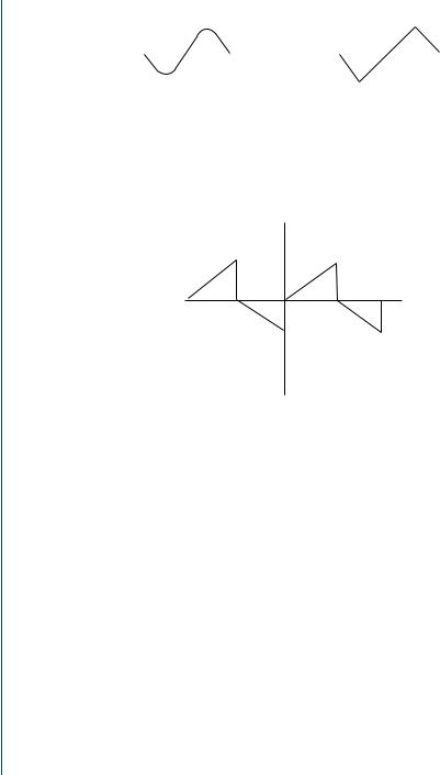
12.4.2 ODD Waveform Symmetries

Similarly, if f (t) satisfies the condition f (t) = − f (−t), then the function is said to

be odd, as shown in Fig. 12.4. The function will contain only the Fourier coefficients bn sin nω0t terms. Note that the functions are folded symmetrically about both y- and x-axes. The negative sign before the time, t, folds the function about the y-axis whereas the negative sign before the function, f , inverts the function about the x-axis.

Another useful property to know is the “half-wave” symmetry. If the function f (t) satisfies the condition f (t) = − f (t ± T2 ), then the function is said to have half-wave symmetry, as shown in Fig. 12.5. The function will contain only the odd complex Fourier

coefficients, an and bn , for n = 1, 3, 5, 7, . . . , etc.

FIGURE 12.3: Another even function. The square wave function is an even function, since the

function is symmetrical about the y -axis, i.e., f (t) = f (−t)

130 SIGNAL PROCESSING OF RANDOM PHYSIOLOGICAL SIGNALS

FIGURE 12.4: Odd functions. The sine wave (a) and the triangular wave are considered to be odd functions since they satisfy the condition f (t) = − f (−t)

FIGURE 12.5: Half-wave symmetric function. This triangular function is considered to have half-wave symmetry since it satisfies the condition f (t) = − f (t ± T2 )

The relationship between the properties of symmetry and the Fourier Series are

summarized in Table 12.10 and as follows:

1.Even functions contain only a0 and an cos nω0t terms.

2.Odd functions contain only bn sin nω0t terms.

3.Half-wave symmetry functions contain only the odd complex Fourier coefficients, an and bn terms, where n = 1, 3, 5, 7, . . . , etc.

Example Problem: What is the Fourier Series of the function, v(t), in Fig. 12.6? The function v(t) is given below.