

Signal Processing of Random Physiological Signals - Charles S. Lessard
.pdfTRUNCATION OF THE INFINITE FOURIER TRANSFORM 161
expect about a 9% error at each region of discontinuity in a signal. It should be noted that discontinuities may occur at the beginning and end points of the analysis window.
Can one correct for the discontinuities and the Gibbs phenomenon? There are a few approaches that may be used. For example, one could use the low-pass filter the signal to remove the high-frequency components, thus smoothing the signal, for example, rounding off the QRS in the electrocardiogram (ECG) signal. Or, one could avoid any analysis in the region of discontinuity by “Piece-meal” or segment analysis.
14.2 SUMMARY
Keep in mind that all Fourier analysis are approximations due to truncation in the number of Fourier coefficients; therefore, from “lessons learned,” one should do the best approximation possible, knowing that 100% accuracy is not attainable. The smoother the signal, the faster it will converge, thus requiring fewer Fourier coefficient terms. Discontinuities either at the edges or in the middle of the signal will result in greater discrepancy (error). Remember that the Gibbs phenomenon indicates that approximately a 9% error will occur in the region of any discontinuity.

163
C H A P T E R 1 5
Spectral Analysis
15.1 INTRODUCTION
Spectral analysis is the process by which we estimate the energy content of a time-varying function (or signal) as a function of frequency. For signals with very little frequency content, the spectral density function can be represented by a “line spectrum.” The variations in the frequency resolution of spectra are due to different window lengths. As the signal becomes more complex (in terms of frequency content), the power spectrum resembles a more continuous function, hence, spectral density functions. The sharp peaks that correspond to the raw estimates of the energy for the main frequency components will be present; however, a certain amount of signal conditioning (i.e., smoothing) is necessary prior to this final estimation of the “Smoothed Power Spectral Estimate.” Notice that at times, the text will refer to the Spectral Density Function as the “Power Spectrum” (singular) or “Power Spectra” (plural). Units for the power spectra are in power per frequency band (spectral resolution, f = 1/ T ).
The harmonic analysis of a random process will yield some frequency information, whereas the power spectrum is a useful tool in analysis of a random process. So let us examine what information can be obtained from the power spectrum. The power spectrum has four major uses. The first is to get an overview of the function’s frequency distribution. Second is for comparison of distribution via statistical testing or by discriminate analysis. Third, the power spectrum can be used to obtain estimates the parameters of interest. And last, but probably the most important application is that power spectra can be used to show hidden periodicities. In summary, spectral estimates are used primarily to

164SIGNAL PROCESSING OF RANDOM PHYSIOLOGICAL SIGNALS
1.show hidden Periodicities in frequency domain;
2.obtain descriptive statistics, for example, distribution, mean, mode, bandwidth of the spectral from a random signal;
3.get an overview of the frequencies in a function, F (ω);
4.in obtaining parameter estimation and/or feature extraction, that is, clinical EEG bands; and
5.in classification testing and discrimination analysis.
There are several methods for calculating the power spectra. The most commonly
used spectral estimation methods are calculated via
1.the autocorrelation function,
2.the direct or fast fourier transform,
3.the autoregression, which is briefly included in this chapter, but this method of spectral estimation will not be covered in the course, since an autoregression course is offered by the statistics department.
It should be noted, however, that there are other methods. The power spectrum (periodogram), most commonly used by engineers, is an estimator of the “raw power spectrum” and must undergo smoothing to clearly reveal informative features (preferred by statisticians). Autoregressive spectral estimation is a powerful tool that estimates the power spectrum without employing any smoothing techniques.
Before commencing with the spectral analysis of a signal, the signal has to be qualified as deterministic (periodic) or random. The random data must be tested for normality of distribution, independence, and stationarity. If any of these statistical properties are not met, the data is a nonstationary process. If the data is nonstationary, appropriate steps should be followed to make the data independent and stationary before proceeding with spectral analysis; however, nonstationary processes are beyond the scope of this book.

SPECTRAL ANALYSIS 165
15.2 SPECTRAL DENSITY ESTIMATION
A basic question one might ask is whether the Fourier Series or transform is applied to a voltage signal, how did the unit become power? To answer this question, let us consider the function v(t) defined over the interval (−∞, +∞). If v(t) is periodic or almost periodic, it can be represented by the Fourier series as in (15.1).
∞ |
|
v(t) = a0 + (an cos nwt + bn sin nwt) |
(15.1) |
1 |
|
where ω = 2π f, f represents the frequency, and the period is T = 1/ f . The complex Fourier coefficients a and b are then represented by equations in (15.2).
|
1 |
|
T |
|
|
a0 = |
|
v(t) d t |
|
||
|
|
|
|||
2T |
0 |
|
|||
|
1 |
|
T |
(15.2) |
|
|
|
v(t) cos(nw0t) d t |
|||
|
|
|
|||
an = 2T |
0 |
||||
|
|||||
|
1 |
|
T |
|
|
bn = |
|
v(t) sin(nw0t) d t |
|
||
|
|
|
|||
2T |
0 |
|
|||
The magnitude of the complex coefficients are obtained from (15.3), which has units of “Voltage/Hertz.”
c n = (an + bn )(an − bn ) |
(15.3) |
The Fourier coefficients are not in units of energy or power. By using Parseval’s Theorem, the power spectrum is obtained from (15.4).
c n2 = an2 + bn2 |
(15.4) |
The squared magnitude of the complex coefficients from (15.4) has units of “Voltage Squared/Hertz,” “Average energy or power per hertz.”
Parseval’s Theorem may be stated as the following equation form (15.5).
+∞ |
v(t) |
2 |
d t = |
1 |
|
|
|
||
−∞ |
|
2π |
||
|
|
|
|
+∞
X(ω) 2 d ω (15.5)
−∞
where v(t) and X(ω) are the Fourier Transform pair.

166 SIGNAL PROCESSING OF RANDOM PHYSIOLOGICAL SIGNALS
The left-hand side of (15.5), is defined as the total energy in the signal v(t).
A periodic signal contains real and imaginary components of power. However, determination of even symmetry (real power only) and odd symmetry (imaginary power only) simplifies calculations because bn and an cancel for each case, respectively. Fourier Series Analysis is a very powerful tool, but it is not applicable to random signals.
15.2.1 Power Spectra Estimation Via the Autocorrelation Function
The classic method used to efficiently obtain the estimated Power Spectra from random processes before the advent of the Fast Fourier Transform was by taking the finite Fourier transform of the correlation function. The process required one to calculate the autocorrelation function (or cross-correlation) first, and then to take the Fourier Transform of the resulting correlation function.
The autocorrelation function (Rx x ) and cross-correlation function (Rx y ) will not be discussed in this section since the material was presented in Chapter 9. Hence, let us assume that the correlation function exists and that its absolute value is finite. The Fourier Transform (FT) is defined as shown in (15.6) for the autocorrelation and (15.7) for the cross-correlation:
Sx x (ω) = |
∞ |
|
Rx x (τ )e − j ωτ d τ |
(15.6) |
|
|
−∞ |
|
Sx y (ω) = |
∞ |
|
Rx y (τ )e − j ωτ d τ |
(15.7) |
|
|
−∞ |
|
where Sx x (ω) is the autospectral density function for an input function x(t), and Sx y (ω) is the cross-spectral density function for the input x(t) and output y (t).
The cross-spectral density function is estimated by taking the cross-correlation of two different functions in the time domain, that is, the input signal to a system and the output signal from the same system, and then taking the Fourier transform of the
resulting cross-correlation function, Sx y . The Inverse Fourier Transforms are then
|
1 |
∞ |
|
Rx x (τ ) = |
|
Sx x (ω)e j ωt d ω |
(15.8) |
2π |
|||
|
|
−∞ |
|

|
|
|
SPECTRAL ANALYSIS 167 |
|
1 |
∞ |
|
Rx y (τ ) = |
|
Sx y (ω)e j ωt d ω |
(15.9) |
2π |
|||
|
|
−∞ |
|
Equations (15.6) through (15.9) are called the “Wiener–Kinchine Relation.”
The Fourier transform of the correlation functions contain real and imaginary components of energy, meaning that the spectrum is a two-sided spectrum with half of the energy containing negative frequencies, that is, −ω; hence, the following equivalent equations are defined in (15.10) and (15.11).
|
|
|
|
Sx x (−ω) = Sx x (ω) = Sx x (ω) |
(15.10) |
||
Sx y (−ω) = |
|
|
(15.11) |
Sx y (ω) = Sx y (ω) |
|||
where the bar over the letter S denotes the complex conjugate.
The S(−ω) and S(ω) are the estimate of the “two-sided spectral density function,” in which the magnitude of the FT for a frequency ω in the real plane is equal to the magnitude of the FT of ω in the imaginary plane. In the case when the autocorrelation function is evaluated over the interval from 0 to ∞, the autospectra may be obtained by using the symmetry properties of the function. An alternate equation is given in (15.12),
with its inverse transform as (15.13).
|
|
|
∞ |
|
|
Sx x (ω) = 2 |
0 |
|
Rx x (τ ) cos(ωτ )d τ |
(15.12) |
|
|
1 |
|
|
∞ |
|
Rx x (τ ) = |
|
|
|
Sx x (ω) cos(ωτ )d ω |
(15.13) |
π |
|
0 |
|||
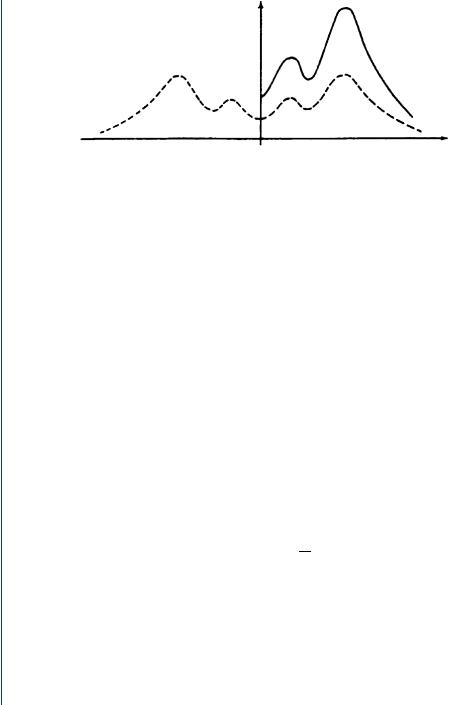
For the case of the “one-sided spectral density function” (Fig. 15.1), in which only the real frequency components of the power spectrum are represented, (15.14) and (15.15) are the same as doubling the energy from one side of the two-sided spectra.
G x x (ω) = 2Sx x (ω) |
(15.14) |
G x y (ω) = 2Sx y (ω) |
(15.15) |
168 SIGNAL PROCESSING OF RANDOM PHYSIOLOGICAL SIGNALS
G(f )
S(f )
f
0
FIGURE 15.1: The two-sided and one-sided spectral density functions
15.2.2 Power Spectra Estimation Directly from the Fourier Transform
With computers and the Fourier transform, it is easier to obtain the spectral estimate directly from the either discrete Fourier transform (DFT) or the fast Fourier transform (FFT). The FFT has become the most popular and widely used method for spectral estimation. The first step in the process requires one to obtain the Fourier coefficients, and then to multiply each coefficient of the autospectrum by its conjugate to get spectral power. The cross-spectral density function is obtained by taking the Fourier transform of the two functions, x(t) and y (t), then the coefficients of one function, X(ω) are multiplied by the conjugate of the coefficients of the second function, Y (ω). The equations for the
ˆ |
ˆ |
|
|||
autospectum (G x x ) and the cross-spectrum (G x y ) are given by (15.16) and (15.17), |
|||||
respectively. The “ˆ” symbol is used to denote a “raw” spectrum. |
|
||||
ˆ |
|
|
|
|
|
(ω) × F 1(ω) |
(15.16) |
||||
G x x = F1 |
|||||
where the “bar” denotes the conjugate of the function.
ˆ |
(ω) × F 2(ω) |
(15.17) |
G x y = F1 |
An alternate method that works well, but only with the autospectrum, is to obtain the Fourier coefficients and calculate the sum of the real term squared, an2, and the imaginary term squared, bn2, as in (15.18). Equation (15.18) should not be used to calculate the cross-spectrum.
ˆ |
2 |
2 |
(15.18) |
G x x = an |
+ bn |
||

SPECTRAL ANALYSIS 169
15.3 CROSS-SPECTRAL ANALYSIS
Cross-spectral analysis is the process for estimating the “Energy” content of “Two” timevarying functions (signals) as a function of frequency. The cross-spectrum has many practical uses in engineering among which the major applications are in
1.determining output/input relationship,
2.obtaining the transfer function of a system from its input and output spectra,
3.determining bode plots from the spectra
a.Magnitude, H(ω)
b.Phase angle, θ (ω),
4.estimating transfer function parameter, and
5.determining “Coherence” or Goodness Fit of the Transfer Function (Model).
The equation for the “one-sided cross-spectral function” from the cross-correlation method is given by (15.19).
G XY ( f ) = 2SXY ( f ) 0 ≤ f < ∞ |
(15.19) |
The expanded form of (15.19) may be expressed as (15.20).
G XY ( f ) = |
∞ |
|
RXY (τ )e − j 2π f τ d τ = C XY ( f ) + j Q XY ( f ) |
(15.20) |
|
|
−∞ |
|
Complex terms of the cross-spectrum are
1.Cx y ( f ) is called the coincident spectral density function (Co-spectrum), and
2.Qx y ( f ) is called the quadrature spectral density function (Quad-spectrum).
Since the cross-spectrum has two terms, a real and an imaginary term, the crossspectrum can be represented in complex polar notation as in (15.21).
G XY ( f ) = G XY ( f ) e − j θXY ( f ) for 0 ≤ f < ∞ |
(15.21) |
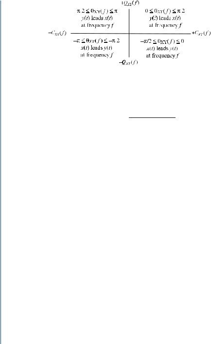
170 SIGNAL PROCESSING OF RANDOM PHYSIOLOGICAL SIGNALS
FIGURE 15.2: The relationship between the phase angle to cross-spectral terms
The magnitude of the cross-spectrum is calculated from (15.22), and the phase is calculated from (15.23).
G XY ( f ) = C XY2 |
( f ) + Q XY2 |
(15.22) |
|
θXY ( f ) = tan−1 |
Q XY ( f ) |
|
(15.23) |
C XY ( f ) |
|||
Special note should be made of the fact that the autospectrum does not retain any phase information whereas the cross-spectrum contains phase information. Keep in mind that engineers look for relationships in both magnitudes or in phase between an input stimulus and the output response of a system. Phase relations are often expressed as leading or lagging a reference signal. The relationship between the phase angle to cross-spectral terms is shown in Fig. 15.2. Since phase is calculated with a tangential function, the relationship is expressed in quadrants.
15.4 PROPERTIES OF SPECTRAL DENSITY FUNCTIONS
For both autospectra and cross-spectra, the Power Spectral Density functions are “Even”
Functions and the Power Spectra are always “Positive” valued functions, G x x > 0.
15.5FACTORS AFFECTING THE SPECTRAL DENSITY FUNCTION ESTIMATION
There are several factors that adversely affect the spectral density function estimation, regardless of the method of estimation that is employed, if these factors are not taken into account.