

Signal Processing of Random Physiological Signals - Charles S. Lessard
.pdf141
C H A P T E R 1 3
Fast Fourier Transform
The “Fast Fourier Transform,” referred to as the “FFT,” is a computational tool that facilitates signal analysis, such as Power Spectral Analysis, by means of digital computers. The FFT is a method for efficiently computing the Discrete Fourier Transform (DFT) of a digitized time series or discrete data samples. The FFT takes advantage of the symmetrical properties of periodic sinusoidal waveforms. Before development of the FFT, transformation of signals into the frequency domain was done by the standard trigonometric Fourier Series computational procedures.
13.1 CONTINUOUS FOURIER TRANSFORM
Before starting on the FFT, let us review or recall from Chapter 12 that the frequency spectrum of an analog signal x(t) may be obtained by taking the Fourier Transform as shown in (13.1):
F (ω) = |
∞ |
|
x(t)e − j ωt dt |
(13.1) |
−∞
where x(t) and F (ω) are complex functions.
13.2 DISCRETE FOURIER TRANSFORM
Also recall that the sampled signal may be written either x(nT ) or x(n),
Sampling
x(t) −−−→ x(nT ) or x(n)
Interval,T

142 SIGNAL PROCESSING OF RANDOM PHYSIOLOGICAL SIGNALS
where T-sampling period and n-number of samples, equally spaced with T as the sampling interval.
Then the Discrete Fourier Transform equation is given by (13.2):
x(ω) = |
∞ |
|
x(n)e − j ωn |
(13.2) |
n=−∞
where ω ranges from 0 to 2π and x(ω) is periodic with 2π
13.3DEFINITION OF SAMPLING RATE (OR SAMPLING FREQUENCY)
Let us review highlights of Chapter 6 on Sampling Theory before discussing the Fast Fourier Transform (FFT). The basis of the Nyquist sampling theorem is the premise that in order to successfully represent and/or recover an original analog signal, the analog signal must be sampled at least twice the highest frequency in the signal. If the highest frequency in the analog signal is known, then it can be sampled at twice the highest frequency, fn · I n terms of time, the spacing between samples is called time period or sampling interval, T. Thus,
T ≤ 1(/2 fn ) or fsampling ≥ 2 fn = 1/ T
where T is the sampling period (or sampling interval), and fsampling is the sampling frequency or sampling rate.
It should be noted that the maximum frequency, fn, is also called the Cutoff Frequency, the Nyquist Frequency, or the Folding Frequency.
If the highest frequency in the signal is not known, then the signal should be bandlimited with an analog low-pass filter, and then the filtered signal should be sampled at least twice the upper frequency limit of the filter bandwidth. If the low-pass filtering procedure is not followed, then the problem of “Aliasing” arises. The Aliasing problem is usually caused when the spacing between samples is very large, which corresponds to sampling at a rate less than twice the highest frequency in the signal.
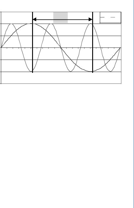
Aliasing is often defined as “the contamination of low frequencies by unwanted high frequency signals/noise” (Fig. 13.1), which by itself is an incorrect statement without
FAST FOURIER TRANSFORM 143
Aliasing at 2 Hz sampling rate
|
1.5 |
|
|
|
|
|
|
|
|
|
|
|
|
|
|
|
|
|
|
|
|
|
|
|
|
|
|
|
|
|
|
T/2 |
|
|
|
|
|
|
|
I Hz |
3 Hz |
||
|
1 |
|
|
|
|
|
|
|
|
|
|
|
|
|
|
|
|
|
|
|
|
|
0.5 |
|
|
|
|
|
|
|
|
|
|
|
|
|
|
|
|
|
|
|
|
Magnitude |
0 |
|
|
|
|
|
|
|
|
|
|
|
|
|
|
|
|
|
|
|
|
|
|
|
|
|
|
|
|
|
|
|
|
|
|
|
|
|
|
|
|
|
|
|
−0.5 |
|
|
|
|
|
|
|
|
|
|
|
|
|
|
|
|
|
|
|
|
|
−1 |
|
|
|
|
|
|
|
|
|
|
|
|
|
|
|
|
|
|
|
|
|
−1.5 |
|
|
|
|
|
|
|
|
|
|
|
|
|
|
|
|
|
|
|
|
|
0 |
0.05 |
0.1 |
0.15 |
0.2 |
0.25 |
0.3 |
0.35 |
0.4 |
0.45 |
0.5 |
0.55 |
0.6 |
0.65 |
0.7 |
0.75 |
0.8 |
0.85 |
0.9 |
0.95 |
1 |
Time (second)
FIGURE 13.1: Aliasing. The example shows that a 3-Hz waveform has the same half period
(T/2) as a 1-Hz waveform, if the signals are sampled at 2 samples per second
some clarification. Aliasing can be eliminated by proper sampling rate (meaning at least twice higher than the highest frequency in the signal) or by low-pass filtering before sampling the signal at a rate not less than twice the known low-pass filter cutoff frequency if the highest frequency in the signal is not known. What is implied by the statement is that if the period of the sampling window is equal to, or less than, one over twice the highest frequency in the signal, T ≤ 1/(2 fn ), then in the frequency domain, the spectrum is repeated every 2π fn Hz. In general, the spectrum repeats over every 2π range from
−∞ to +∞. Thus, it would be sufficient to obtain values between 0 and 2π in a DFT.
13.3.1 Short-Hand Notation of the Discrete Fourier Transform (DFT)
The DFT is often written as in (13.3).
N−1 |
|
x(k) = x(n)WNnk for k = 0, 1, . . . , N − 1 |
(13.3) |
n=0 |
|

144 SIGNAL PROCESSING OF RANDOM PHYSIOLOGICAL SIGNALS
TABLE 13.1: Spectral Window vs. Frequency Resolution
|
fsampling rate |
N |
T |
|
|
|
|
1. |
1 sec − 2000 samples/sec |
2000 |
0.0005 |
2. |
1 sec − 1000 samples/sec |
1000 |
0.001 |
3. |
2 sec − 1000 samples/sec |
2000 |
0.05 |
Since wn = 2π/N = 2π T. The frequency resolutions are shown below.
1. |
0.003141592 |
fres = |
ω0 |
|
=1.0 Hz |
|
2π T |
||||||
2. |
0.006283185 |
fres = |
ωn fsamp |
=1.0 Hz |
||
|
2π |
|||||
3. |
0.00314592 |
|
|
|
|
=0.5 Hz |
where WN = e − j 2π/N is called phase or The Twiddle Factor, x(k) is called the N-point DFT, and the distance between successive samples in the frequency domain gives the fundamental frequency of x(t).
In terms of normalized frequency units, the fundamental frequency is given by 2π/N. Note in the example given in Table 13.1 that a one-second window results in a
1-Hz frequency resolution regardless of the sampling rate.
By definition, the Frequency Resolution ( fres) or the fundamental frequency of the spectral ( f0) is “The minimum frequency that a signal can be resolved in the frequency domain, and is equal to the inverse of the record length or the signal window length
being analyzed (in seconds) in time domain” (13.4): |
|
||||
fres = |
1 |
= |
1 |
|
(13.4) |
|
|
|
|||
R.L |
N T |
||||
Record length: The length of the sampled analog signal with a total of N samples is given
as R.L = NT.
Expanding the DFT equation results in (13.5):
N−1 |
{(Re[x(n)]Re[WNnk ] − Im[x(n)]Im[WNnk ]) |
x(k) = |
|
n=0N |
(13.5) |
+ (Re[x(n)]Im[WNnk ] + Im[x(n)]Re[WNnk ])} where k = 0, 1, . . . , N − 1

FAST FOURIER TRANSFORM 145
W 3 |
W 2 |
W 1 |
8 |
8 |
8 |
W 4 |
W 0 |
8 |
8 |
W 5 |
W |
6 |
W 7 |
8 |
|
8 |
8 |
FIGURE 13.2: Symmetry and periodicity of WN for N = 8
For each k, (13.5) needs 4N real multiplications and (4N − 2) real additions. The computation of x(k) needs 4N 2 real multiplications and N(4N − 2) real additions. In terms of complex operations, there are N 2 complex multiplication and N(N − 1) complex additions. As N increases, it can be seen that the number of computations become tremendously large. Hence, there was a need to improve the efficiency of DFT computation and to exploit the symmetry and periodicity properties of the twiddle factor,
WN , as shown in (13.6) and Fig. 13.2.
Symmetry : WNk |
= −WNk+ N2 |
(13.6) |
Periodicity : WNk |
= WNN+k |
|
13.4 COOLEY-TUKEY FFT (DECIMIMATION IN TIME)
The Cooley–Tukey FFT was one of the first FFTs developed. Suppose a time series having N samples is divided into two functions, of which each function has only half of the data points (N/2). One function consists of the even numbered data points (x0, x2, x4 . . . , etc,), and the other function consists of the odd numbered data points (x1, x3, x5, . . . , etc.). Those functions may be written as
Yk = x2k ; Zk = x2k+l , for: k = 0, 1, 2, . . . , (N/2) − 1
Since Yk and Zk are sequences of N/2 points each, the two sequences have Discrete Fourier transforms, which are written in terms of the odd and even numbered data points. For values of r greater than N/2, the discrete Fourier transforms Br and Cr repeat

146 SIGNAL PROCESSING OF RANDOM PHYSIOLOGICAL SIGNALS
periodically the values taken on when r < N/2. Therefore, substituting r + N/2 for r in (13.7), one can obtain (13.8) by using the Twiddle Factor, W = exp(−2π j /N).
Ar = Br + W r Cr |
(13.7) |
Ar + N2 = Br − W r Cr |
(13.8) |
From (13.7) and (13.8), the first N/2 and last N/2 points of the discrete Fourier transform of the data xk can be simply obtained from the DFT of both sequences of N/2 samples. Assuming that one has a method that computes DFTs in a time proportional to the square of the number of samples, the algorithm can be used to compute the transforms of the odd and even data sequences using the Ar (13.7) and Ar + N/2 (13.8) equations to find Ar. The N operations require a time proportional to 2(N/2)2.
Since it has been shown that the computation of the DFT of N samples can be reduced to computing the DFTs of two sequences of N/2 samples, the computation of the sequence Bk or Ck can be reduced by decimation in time to the computation of sequences of N/4 samples. These reductions can be carried out as long as each function has a number of samples that are divisible by 2. Thus, if N = 2n , n such reductions (often referred to as “Stages”) can be made.
For example, the successive decimation (reduction) of a Discrete Fourier Transform will result in a Fast Fourier Transform with fewer computations. In general, N log2 N complex additions and at most (1/2)N log2 N complex multiplications are required for computation of the Fast Fourier Transform of an N point sequence, where N is a power of 2 (N = 2n ).
13.4.1 Derivation of FFT Algorithm
Consider the N-point DFT that can be reduced into two N/2 DFTs (even and odd indexed sequences), as x(n) is decomposed into two N/2-point sequences (decimation- in-time) and is shown in (13.9).
N2 −1 |
x(2n)WN2nk + |
N2 −1 |
|
··· x(k) = |
x(2n + 1)WN(2n+1)k |
(13.9) |
|
n=0 |
|
n=0 |
|

FAST FOURIER TRANSFORM 147
2 |
= |
e |
− j |
2π 2 |
= e |
− j |
2π |
= W |
|
N |
(N/2) |
N |
|||||||
where: WN |
|
|
|
|
2 |
Then, (13.9) can then be rewritten as (13.10).
|
|
|
N2 −1 |
x(2n)W nkN |
|
W k |
N2 −1 |
|
1)W Nnk |
|
· |
· |
x(k) |
= |
+ |
x(2n |
+ |
(13.10) |
|||
· |
|
2 |
N |
n=0 |
2 |
|
||||
|
|
|
n=0 |
|
|
|
|
|
|
where x1(k) is = x1(k) + WNk x2(k), k = 0, 1 . . . , N.
The sequences, x1(k) and x2(k) can each be further divided into even and odd sequences as shown in (13.11) and (13.12).
N2 |
−1 |
x (2n) WNnk/2, |
for |
k = 0, 1, . . . , |
N |
− 1 |
|
|
(13.11) |
||||
x1 (k) = |
|
|
|
|
|
|
|||||||
|
2 |
|
|
|
|
||||||||
n=0 |
|
|
|
|
|
|
|
|
|
|
|
|
|
N4 |
−1 |
nk |
|
k |
N4 −1 |
nk |
|
|
|
|
N |
− 1 |
|
|
|
|
|
|
|
|
|
||||||
= n=0 |
x (4n)WN/4 |
+ WN/2 n=0 |
x (4n + 2) WN/4 |
, |
for |
k = 0, 1, . . . , |
|
||||||
4 |
|||||||||||||
and for the x2(k) sequence as shown in (13.13) and (13.14):
N2 |
−1 |
nk |
|
|
|
N |
|
|
|
|
|
|
|
|
|||
x2 (k) = |
|
x (2n + 1) WN/2 |
, for |
k = 0, 1, . . . , |
|
|
− 1 |
|
|
2 |
|||||||
n=0 |
|
|
|
|
|
|
|
|
N4 |
−1 |
nk |
k |
N4 −1 |
|
nk |
|
|
= n=0 |
|
|
|
|||||
x (4n + 1) WN/4 |
+ WN/2 n=0 |
x (4n + 3) WN/4 |
, for |
|||||
(13.12)
(13.13)
k = 0, 1, . . . , N4 −1 (13.14)
Table 13.2 shows the reduction in computations between the DFT and the FFT.
TABLE 13.2: Comparison DFT and FFT Computation with N = 8
COMPLEX |
DFT |
FFT |
colruleMultiplications |
N 2 = 64 |
N log2 N = 24 |
Additions |
N (N − 1) = 56 |
N log2 1 = 24 |
|
For N = 65 536 |
|
Complex multiplications |
4.3 × 10⁹ |
1.049 × 10⁶ |
148 SIGNAL PROCESSING OF RANDOM PHYSIOLOGICAL SIGNALS
Xm( p) |
1 |
|
|
Xm+1( p) |
|
|
|
||
|
|
|
|
WNr |
Xm( q) |
|
|
|
1 |
WNr+N/2 |
|
|
Xm+1( q) |
|
|
|
|
|
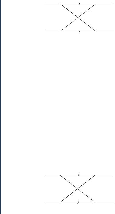
FIGURE 13.3: FFT “Butterfly” signal flow diagram
13.5 THE FFT “BUTTERFLY” SIGNAL FLOW DIAGRAM
To predict the next value in the stage (decimation), the previous stage values are used as inputs, where p may indicate the odd sequence and q the even sequence. The flow graph (Fig. 13.3) is called the “butterfly computation” because of its appearance.
The output of the stage is calculated with (13.15) and (13.16).
Xm+1 ( p) = Xm ( p) + WNr Xm (q ) |
(13.15) |
Xm+1 (q ) = Xm ( p) + WNr + N2 Xm (q ) |
(13.16) |
However, from symmetry and periodicity properties:
N |
) = e − j π = −1 |
WN2 = e − j ( 2Nπ )( N2 |
the reduced Butterfly flow diagram becomes Fig. 13.4 and the equations are rewritten as
Xm( p) |
1 |
|
|
Xm+1( p) |
|
|
|
||
|
1 |
|||
Xm( q) |
|
|
1 |
|
|
|
|
Xm+1( q) |
|
|
−1 |
|||
FIGURE 13.4: Reduced Butterfly flow diagram

FAST FOURIER TRANSFORM 149
(13.17) and (13.18). |
|
Xm+1 ( p) = Xm ( p) + WNr Xm (q ) |
(13.17) |
Xm+1 (q ) = Xm ( p) − WNr Xm (q ) |
(13.18) |
Bit Reversal : To perform the computation as shown in the Fig. 13.4 flow graph, the input data must be stored in a nonsequential order and is known as the bit-reverse order. For a sequence of N = 8, the input data are represented in binary form as
LSB = 0
X (0) = X (0, 0, 0)
X (4) = X (1, 0, 0)
X (2) = X (0, 1, 0)
X (6) = X (1, 1, 0)
LSB = 1
X (1) = X (0, 0, 1)
X (5) = X (1, 0, 1)
X (3) = X (0, 1, 1)
X (7) = X (1, 1, 1)
Upon observation, one can see that the bits (LSB = 0) of the top section are all even number samples; and LSB = 1 of bottom section are all odd number samples, which are obtained by writing the signal sequences in binary form and bit-reversing each to get the new order. If the input is not bit-reversed, then the output will need to be bit-reversed. The flow graph can be arranged in such a way that both input and output need not be bit-reversed.
13.6 DECIMATION-IN-FREQUENCY
The configuration is obtained by dividing the output sequence into smaller and smaller subsequences. Here the input sequence is divided into first or second halves. According to Fourier integral theorem, a function must satisfy the Dirichlet conditions or every finite interval and the integral from infinity to negative infinity is finite. The
150 SIGNAL PROCESSING OF RANDOM PHYSIOLOGICAL SIGNALS
conditions are
1)the function should have a finite number of maxima or minima,
2)the function should have a finite number of discontinuities, and
t−T
3) the function should have a finite value or |
f (t) d t is less than infinity. |
t
Conditions for the Fourier Series include the following:
1)periodic functions (practical is nonperiodic);
2)can only be applied to stable systems (systems where natural response decays in time, for example, convergent).
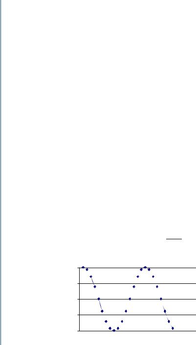
Example Problem : Consider the sinusoidal waveform of Fig. 13.5.
According to Nyquist sampling theorem, the waveform in Fig. 13.5 should be sampled at more than two samples per second to successfully reconstruct the signal. For the sake of convenience, consider eight samples per second of the above waveform. Therefore: N = 8 = 2n = 23, N is the total number of samples, and n = 3 stages;
T = 125 milliseconds, sampling interval; Record length = 1 second (time of recording data = N × T) Frequency resolution = 1 Hz (1/(N × T ))
The discrete signal is given by (13.19).
X (nT ) = cos |
2πfnT |
= cos |
2π fn |
(13.19) |
N |
||||
1 |
|
|
|
|
0.5 |
|
|
|
|
0 |
|
|
|
|
−0.5 |
|
|
|
|
−1 |
|
|
|
|
FIGURE 13.5: Trace of the waveform is x (t) = cos (ωt), where ω = 2π f and f = 1 Hz |
||||