

Signal Processing of Random Physiological Signals - Charles S. Lessard
.pdfCONVOLUTION 91
a
|
|
|
|
|
|
0 |
|
t |
|
-u(a - t)
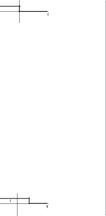
FIGURE 10.12: Combining the operations of folding and translating about both axes. The step
function folded about both axes and displaced by +a gives the unit step function expressed as
−u(a − t)
Combining the operations of folding about the y-axis, then folding about the x- axis, and translating the step function by a positive displacement of +a gives the results shown in Fig. 10.12. The unit step function is then expressed as −u(a − t).
10.1.1Real Translation Theorem
One can summarize the operation of translation along an axis by a well-known theorem which states that any function f (t), delayed in its beginning to some time t = a , can be represented as a time-shifted function as in (10.9).
f (t − a ) μ (t − a ) |
(10.9) |
where μ(t − a ) =
1, −t ≥ a
0, −t < a
Proof of the time shift theorem is based in LaPlace Transform of the two functions, which is often referred to as the Real Translation Theorem or simply the Shifting Theorem as shown in the resulting (10.10).
L [μ (t − a )] = |
e −a s |
|
(10.10) |
|
|
s |
|||
where, e −a s shifts the transform from t = 0 to t = ∞. |
|
|||
Let us return to the visualization of convolution. The function f (τ ) should not be |
||||
a problem since it is similar to the function f (t), |
|
except for the change of independent |
||
variable from units of time t to units of delay τ . |
It is important to keep in mind that |
|||
once the variable is changed from time t to delay τ |
that the unit of delay τ |
becomes the |
||
independent variable and that time t in the function f (t − τ ) is the same as displacement a in the function f (a−t).

92 SIGNAL PROCESSING OF RANDOM PHYSIOLOGICAL SIGNALS
f (t )
0 t
FIGURE 10.13: Simple unity step function
Before discussing the complete process of convolution, the reader should know that calculation of the convolution requires the following steps, which were previously described.
1.Change of variable from time, t, to delay, τ
2.Folding about the vertical axis
3.Translation
Let us look at an example, using the three steps to visualize and examine the process with a simple function, f (t), as shown in Figs. 10.13–10.16.
The first step in the convolution process is the change of independent variable from a function of time, f (t), to a function of delay, f (τ ), as in Fig. 10.14.
The second step is to fold the step function about the y-axis, f (−λ), as in Fig. 10.15.
The third step is to translate the step function along the x-axis some distance, t, as shown in Fig. 10.16. Note that the folded and translated step function is written as f (t − τ ).
Let us examine another example; assume the function f (t) = Ae −a t . Figure 10.17 shows the function and the first step, which is the change of variable.
f ( )
0
FIGURE 10.14: First step. Change the independent variable from a function of time, f (t), to a
function of delay, f (τ )
CONVOLUTION 93
f (– )
)
0
FIGURE 10.15: Second step. The step function is folded about the y-axis, f (−λ)
Figure 10.18 shows the folding and translation steps. Note that the translation is to the right. The function f (t − τ ) can be thought of as f {−(τ − t)}, then f (−τ ) where τ is (τ − t), which results in movement to the right (positive direction).
In the next example, illustrated in Fig. 10.19, the original does not begin at t = 0, but is delayed by some magnitude a. The amount of displacement of the function is measured from the position of f (−τ ) which is f (t − τ ) at t = 0. Note that the amount of delay is carried in the folding about the y-axis, which implies that the zero values must be accounted for in calculation of the convolution integral.
10.1.2Steps in the Complete Convolution Process
The entire process of convolution requires the five steps listed as follows:
1.Change of variable
2.Folding about the vertical y-axis
3.Translation along the horizontal x-axis
4.Multiplication of the two functions, f1(τ ) and f2(t − τ )
5.Integration of areas
The process might be synopsized as determining the area under the curves (product) as the folded function is slid along the horizontal axis. Note the direction of translation; the conventional notation is as follows:
f (– )
0
FIGURE 10.16: Third step. Translation of the function along the x-axis some distance, t
94 SIGNAL PROCESSING OF RANDOM PHYSIOLOGICAL SIGNALS
|
|
|
f (t) |
|
|
|
|
|
|
f ( ) |
|||||||||
|
|
|
|
|
|
|
|
|
|||||||||||
|
|
|
|
|
|
|
|
|
|||||||||||
|
|
|
|
|
|
|
|
|
|
|
|
|
|
|
|
|
|
|
|
|
|
|
|
|
|
|
|
|
|
|
|
|
|
|
|
|
|
|
|
|
|
|
|
|
|
|
|
|
|
|
|
|
|
|
|
|
|
|
|
|
|
0 |
|
|
|
t |
0 |
|
|
|
|
|
|
|
|
|
|||
|
|
|
|
|
|
|
|
|
|||||||||||
|
|
(a) Original function |
|
|
|
|
(b) Change of variable |
||||||||||||
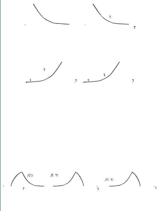
FIGURE 10.17: First step. (a) It shows the original function f (t) = Ae −a t . (b) It shows the change of variable for the function
|
|
|
|
|
|
|
|
|
|
|
|
|
|
|
|
|
|
|
|
|
|
|
|
|
|
|
|
|
|
|
f (– ) |
|
|
|
|
|
|
|
|
|
|
|
|
|
|
|
|
|
|
|
|
||||
|
|
|
|
|
|
|
|
|
|
|
|
|
|
|
|
|
|
|
f (– ) |
|
|
|
|
||||
|
|
|
|
|
|
|
|
0 |
|
|
|
|
|
|
|
|
|
|
|
0 |
|
|
|
||||
|
|
|
|
|
|
|
|
|
|
|
|||||||||||||||||
|
|
|
|
|
|
|
|
|
|
|
|
|
|
|
|
|
|
|
|
|
|
|
|
|
|
||
|
|
|
(a) Folding |
|
|
|
|
|
|
|
|
|
|
|
|
|
|||||||||||
|
|
|
(b) Translation |
||||||||||||||||||||||||
FIGURE 10.18: Next two steps. (a) It shows folding of the function about the y-axis and (b) it shows the translation step
a.Movement to the right for positive (+) time
b.Movement to the left for negative (−) time
Let us visualize an example, in which two functions of unity magnitude are to be convolved. Assume the two functions are given by (10.11) and (10.12).
f1(t) = 1μ(t) |
(10.11) |
|
|
|
|
|
|
|
|
|
|
|
|
|
|
|
|
|
|
|
|
|
|
|
|
|
|
|
|
|
|
|
|
|
|
|
|
|
|
|
|
|
|
|
|
|
|
|
|
|
|
|
|
|
|
|
|
|
|
|
|
|
|
|
|
|
0 a |
b |
|
|
–b |
–a |
|
0 |
(t–b) |
|
|
0 (t–a) |
|||||||
|
|
|
||||||||||||||||||
|
|
|
(a) Original |
|
|
|
|
|
(b) Folded |
|
|
|
|
|
|
(c) Translated |
||||
FIGURE 10.19: Another Example. It should be noted that the original does not begin at t = 0, but is delayed by some magnitude a. Figures 10.19(a) through (c) show that the amount of delay is carried through the Folding and Translation steps

CONVOLUTION 95
f1

f2

0 |
0 |
FIGURE 10.20: First step. Graphs of the two equations are shown after changing the indepen-
dent variable
and
f2(t) = e −a t |
(10.12) |
After changing the independent variable from time t to delay τ , the expressions are written as functions of τ , which are given in (10.13) and (10.14).
f1(τ ) = μ(τ ) |
(10.13) |
and |
|
f2(τ ) = e −a τ |
(10.14) |
Graphs of the two equations are shown in Fig. 10.20.
The next step is to fold one of the two functions about the y-axis. Either variable may be folded, since the results will be the same. In this case the step function was selected as the function to fold. Thus, f1(τ ) = μ(τ ) becomes f1(−τ ) = μ(−τ ) as shown in Fig. 10.21. Note that the second function, f2(τ ) = e −a τ , remains the same.
|
|
|
|
|
|
|
|
|
|
|
|
f2 |
|||
|
|
|
|
|
|
|
|
|
|
|
|
||||
|
|
|
|
|
|
|
|
|
|
|
|
||||
|
|
|
|
|
|
|
|
|
|
|
|
||||
|
|
|
|
|
|
|
|
|
|
|
|
||||
|
|
|
|
|
|
|
|
|
|
|
|
|
|
|
|
|
|
|
|
|
|
|
|
|
|
|
|
|
|
|
|
|
|
|
|
|
|
|
|
|
|
|
|
|
|
|
|
|
|
|
|
|
|
|
|
|
|
|
|
|
|
|
|
0 |
0 |
|
|
|
|
||||||||||
(a) f1 folded |
|
|
|
|
|
|
(b) f2 not folded |
||||||||
FIGURE 10.21: Function f1 Folded. The step function in Fig. (a) was folded while the second function was not folded

96 SIGNAL PROCESSING OF RANDOM PHYSIOLOGICAL SIGNALS
0 |
t1 |
t2 |
0 |
t1 |
t2 |
(a) Translation, product, and integration |
(b) Resulting convolved function |
FIGURE 10.22: Last three steps. The final steps of translation, product, and integration in the
convolution process are shown in (a) with the resulting function shown in (b)
The final steps of translation, product, and integration in the convolution process are shown in Fig. 10.22(a) with the final convolution function being shown in Fig. 22(b). The reader should keep in mind that the integrated product is the same as the area under the product graph. In the first translation (t1 ), the integrated quotient is shown as the area with the cross hatches slanting downward to the right. The new area of the integrated quotient for the second translation (t2) is shown with the cross hatches slanting upward to the right. Note in the results, shown in Fig. 10.22(b), that the result at t2 is the total area (both cross-hatched areas). The action of the functions f1 and f2 on each other is thought of as a smoothing or weighting operation.
Let us examine the convolution of a pulse and another function: assume the functions are defined as follows and are described by (10.15) and (10.16).
1.f1(t) is a rectangular pulse of height 3 and width 2
2.f2(t) is an exponential decay height 2 at t = 0
f1 (t) = 3 [μ (t) − μ (t − 2)] |
(10.15) |
f2 (t) = 2e −2t μ (t) |
(10.16) |
where f2(t) = 0 for t < 0. |
|
Evaluation of the convolution integral is given by (10.17). |
|
∞ |
|
f3 = f1 (t) × f2 (t) = 6 [μ (t − τ ) − μ (t − 2 − τ )] e −2τ μ (τ ) ∂ τ |
(10.17) |
−∞ |
|
CONVOLUTION 97
f1(t ) |
3 |
|
f1 |
2 |
|
|
|
|
|
|
f2(t ) |
0 |
2 |
t |
FIGURE 10.23: Second step: Folding. The figure shows the two functions after folding the
pulse. It should be noted that there is no overlap of the functions when t ≤ 0
Figure 10.23 shows the two functions after folding the pulse; note that at the start, when t ≤ 0, there is no overlap and the resulting value of the convolution integral ( f3 ) at t = 0 is zero, ( f3 = 0).
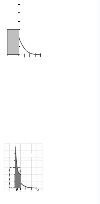
Following the folding step, the exponential function, f2 , is multiplied by the pulse function, f1 , with a magnitude of 3, then the area between 0 < t < 1 is integrated. The result of the integration is the first value of the convolution function, f3 , which is the shaded area in Fig. 10.24.
6
f2(t)
2
0 |
|
t |
FIGURE 10.24: Result of integration. The first value of the convolution function, f3 , is shown by the shaded area in the figure
98 SIGNAL PROCESSING OF RANDOM PHYSIOLOGICAL SIGNALS
6
f2(t)
4
2
0 |
|
2 |
|
t |
|
|
|
|
|
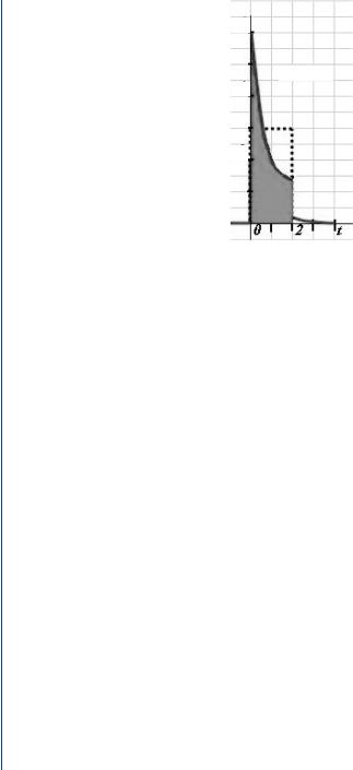
FIGURE 10.25: Result from the second translation. The second value after integration of the
convolution function, f3 , with the limits between 0 < t < 2, is shown by the shaded area in the figure
The next step is to repeat the translation step by moving the pulse function one increment to the right; hence, the limits of integration are changed to the interval of 0 < t < 2, as given by (10.18).
t |
|
f3 (t) = 6 e −2τ ∂ τ |
(10.18) |
0 |
|
The result of the second translation and including the multiplication and integration steps is shown in Fig. 10.25. Note that the width of the area is equal to the width of the pulse function. As the pulse is translated to the next interval between 0 < t < 3, it should be noted that the common area is reduced to the interval between 1 < t < 3 (the width of the pulse). Hence, for this example, the area is smaller than the previous one. As the pulse is continuously translated, the value of the integrated area approaches zero.
The process repeats the three steps:
1.Translation along the horizontal x-axis
2.Multiplication of the two functions, f1 (τ ) and f2 (t − τ )
3.Integration of area bound by the limits of integration

CONVOLUTION 99
In the example, for the next translations the limits are reset to the interval between 2 < t < ∞ as shown in (10.19).
t |
|
f3 (t) = 6 e −2τ ∂ τ |
(10.19) |
t−2
10.1.3Convolution as a Summation
In evaluation of the convolution integral by digital computer, it is necessary to replace the integral (10.20) with a finite summation.
t |
|
v2 (t) = v1 (τ ) h (t − τ ) ∂ τ |
(10.20) |
0 |
|
To accomplish this conversion, the infinitesimal ∂ τ is replaced with a time interval of finite width T and τ is replaced with nT. The convolution integral is written as the summation for K T ≤ t < (K + 1)T as shown in (10.21).
K |
|
v2 (t) = T v1 (nT) h (t − nT ) |
(10.21) |
n=0 |
|
where K is one of the values of the integer n. |
|
Equation (10.22) gives the convolution of (10.21) in expanded form. |
|
v2(t) = T [v1 (0) h (t) + v1(T )h (t − T ) |
|
+ v1(2T )h (t − 2T ) + v13T )h (t − 3T ) + · · ·] |
(10.22) |
Each term in (10.22) is the impulse response of magnitude of v1 (nT ) shifted along the t-axis and later is multiplied by T. Summation of the terms in the equation approximates the function. The accuracy of the approximation will depend on the magnitude of T. The smaller the value of T is, the better the approximation.
10.2NUMERICAL CONVOLUTION
Numerical evaluation of the convolution integral is straightforward. When either function is of finite duration, there will be a finite number of terms in each summation.

100 SIGNAL PROCESSING OF RANDOM PHYSIOLOGICAL SIGNALS
However, when the functions are of infinite duration, the computations become lengthy as the overlapped area becomes very large. There are alternative methods that can be applied for simple problems or when a computer is available.
10.2.1Direct Calculation
10.2.1.1 Strips of Paper Method
One of the numerical methods is to use two strips of paper and to follow the following steps:
1.tabulate values of the two functions at equally spaced intervals on two strips of paper;
2.reverse tabulate one function; f (−λ), which is equivalent to folding a function;
3.place strips beside each other and multiply across the strips and write the products;
4.slide one strip, and repeat step three, until there are no more products;
5.sum the rows; and
6.multiply each sum by the interval width.
10.2.1.2 Polynomial Multiplication Method
Another method is the polynomial multiplication method (Table 10.1). For this method, the values of the two functions are placed in two rows one function above the other (without any reverse tabulation) as in Table 10.1. It should be noted that the functions are aligned to the left and not to the right as in normal multiplication. The alignment and multiplication from left to right serves as equivalence to folding of a function about the y-axis. The number of terms in the results should equal the sum of the number of terms in the two functions. The final results of the convolution operation are obtained by summing the columns and multiplying the resulting summations by the interval width.
At this point, it is worth discussing an area of possible confusion: that of establishing the proper relationship of the time variable to the sample values employed in the