Signal Processing of Random Physiological Signals - Charles S. Lessard

WINDOW FUNCTIONS AND SPECTRAL LEAKAGE 191

From trigonometric identities, an alternate method for expressing the cosine window is to write the expression in terms of the “Sine” function, when the data are not symmetrical about the origin. For example if α = 2 the cosine model becomes as shown in by (16.5).

16.3.6 Welch Window

This window is a modification of the Parzen window with some better characteristics especially in the coherent gain; however, the Welch window produces greater main lobe leakage due to a wider spreading. The mathematical model for the Welch window is given by (16.7). Notice the polynomial similarity between Parzen and Welch expressions.

This type of window is not good for signals with closely related spectral components. The main side-lobe effect can be worse than the leakage from the rectangular

window.

16.3.7 Blackman Window

The name “Blackman Window” was given to honor Dr. Blackman, a pioneer in the harmonic signal detection. There are several windows under his name, differing in the amount of variables used. For simplicity only the “Exact Blackman Window” will be described, since this window has superb tone discrimination characteristics (used in

where n = −N/2, . . . . , −1, 0, +1, . . . . , +N/2

WINDOW FUNCTIONS AND SPECTRAL LEAKAGE 193

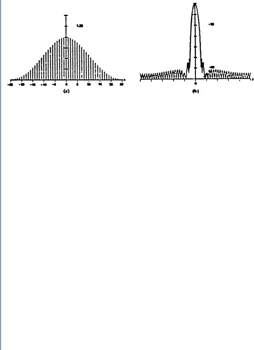
The effects of leakage can be suppressed or reduced with the application of special functions called “Windows.” As many as 58 window functions have been developed with various optimizations in mind. In practice, most engineers will apply a Hanning or Hamming window; however, it is not recommended that only one window be used for all applications, but rather that several windows should be tried for the best results in the particular situation.

16.5REFERENCES

1.Bendat, J., and Piersol, A. Randon Data Analysis and Measurement Procedures, 2nd Edition, Wiley, pp. 393–400.

2.Gabel, R., and Roberts, R. Signals and Linear Systems, pp. 253–370.

3.Flannery, B., Tenkolsky, S., and Veterling, W. Numerical Recipes: The Art of Scientific Computing. Wesley Press, pp. 381–429.

4.Van Valkenburg, M. E. Network Analysis, pp. 452–495.

16.6SUGGESTED READING

1.Bergland, G. D. “A Guided Tour of the Fast Fourier Transform,” IEEE Spectrum, pp. 41–52, July 1969.

2.Harris, F. “The use of Windows for Harmonic Analysis with DFT,” Proceedings of IEEE, Vol. 6, No. 1, January 1978.

3.Geckinki, N., and Yanuz, D. IEEE Transactions on Acoustics Speech and Signal Processing. Vol. 26, No. 6, December 1978.

4.Nudall, A. “Some Windows With Very Good Sidelobe Behavior,” IEEE Transactions on Acoustics Speech and Signal Processing, Vol. 29, No. 1, February 1981.

195

C H A P T E R 1 7

Transfer Function Via

Spectral Analysis

17.1 INTRODUCTION

This chapter describes the method for estimation of the frequency response of a linear system, using spectral density functions. The autocorrelation and cross-correlation functions are discussed to provide background for the development of their frequency domain counterparts, the autospectral and cross-spectral density functions. The coherence function is also discussed as a means of calculating the error in the transfer function estimation. Applications will be restricted to single input/single output models, where it is assumed that systems are constant-parameter, linear types.

To meet control system specifications, a designer needs to know the time response of the controlled variable in the system. Deriving and solving the differential equations of the system can obtain an accurate description of the system’s response characteristics; however, this method is not particularly practical for anything but very simple systems. With this solution, it is very difficult to go back and decide what parameters need to be adjusted if the performance specifications are not met. For this reason, the engineer would like to be able to predict the performance of the system without solving its associated differential equations and he/she would like for his/her analysis to show which parameters need to be adjusted or altered in order to meet the desired performance characteristics.

The transfer function defines the operation of a linear system and can be expressed as the ratio of the output variable to the input variable as shown in Fig. 17.1.

196 SIGNAL PROCESSING OF RANDOM PHYSIOLOGICAL SIGNALS

FIGURE 17.1: Transfer function from input–output

The common approach to system analysis is to determine the system’s transfer function through observation of its response to a predetermined excitation signal. Evaluation of the system characteristics can be performed in the time or frequency domains.

17.2 METHODS

The engineer has several methods available to him/her for evaluating the system’s response. The Root Locus Method is a graphical approach in the time domain, which gives an indication of the effect of adjustment based on the relation between the poles of the transient response function, and the poles and zeros of the open loop transfer function. The roots of the characteristic equation are obtained directly to give a complete solution for the time response of the system.

In many cases it is advantageous to obtain system performance characteristics in terms of response at particular frequencies. Two graphical representations for transfer function derivations are the Bode and Nyquist Methods. The Bode Plot Method yields a plot of the magnitude of the output/input ratio versus frequency in rectangular or logarithmic coordinates. A plot of the corresponding phase angle versus frequency is also produced. The Nyquist Plot Method is very similar: it plots the output/input ratio against frequency in polar coordinates. The amplitude and phase data produced with these methods are very useful for obtaining an estimate of the system’s transfer function. They can be determined experimentally for a steady-state sinusoidal input at various frequencies, from which the magnitude and phase angle diagrams are then derived directly, leading to the synthesis of the transfer function.

Analytical techniques that fit rational polynomial transfer functions using digital computers are very popular as they speed the evaluation process considerably. In the next section, two functions, which provide analytical methods for measuring the time-domain properties of signal waveforms, will be developed.

TRANSFER FUNCTION VIA SPECTRAL ANALYSIS 197

17.3 AUTOCORRELATION

The autocorrelation function gives an average measure of the time-domain properties of a signal waveform. It is defined as (17.1):

f (t + τ ). The expression above applies to the case of a continuous signal of infinite duration. In practice, the intervals must be finite and it is necessary to use a modified

version as given by (17.2).

∞

The autocorrelation function may be applied to deterministic as well as random signals. Each of the frequency components in the signal f (t) produces a corresponding term in the autocorrelation function having the same period in the time-shifted variable,

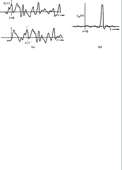
τ , as the original component has in the time variable, t. The amplitude is equal to half of the squared value of the original. The phase shifts of each signal produce a single cosine term in the autocorrelation as shown in Fig. 17.2.

FIGURE 17.2: Autocorrelation. Trace (b) is the autocorrelation of the signal shown in (a)

198 SIGNAL PROCESSING OF RANDOM PHYSIOLOGICAL SIGNALS

The fact that the autocorrelation is composed of cosines implies that it must be an even function of τ . When τ = 0, all of the cosine functions reinforce each other to give a peak positive value for the autocorrelation. Whether this peak value is ever attained for other shifts of τ depends on whether the components of the signal are harmonically related or not. The peak value of the autocorrelation function at τ = 0 is simply the mean square value, or average power of the signal, and is given by (17.3) [1].

17.4 THE CROSS-CORRELATION FUNCTION

The cross-correlation function is essentially a time-averaged measure of shared signal properties and is defined as (17.4).

where τ is a time shift on one of the signals. Since signals to be compared must be of finite duration, the function is modified as shown in (17.5).

∞

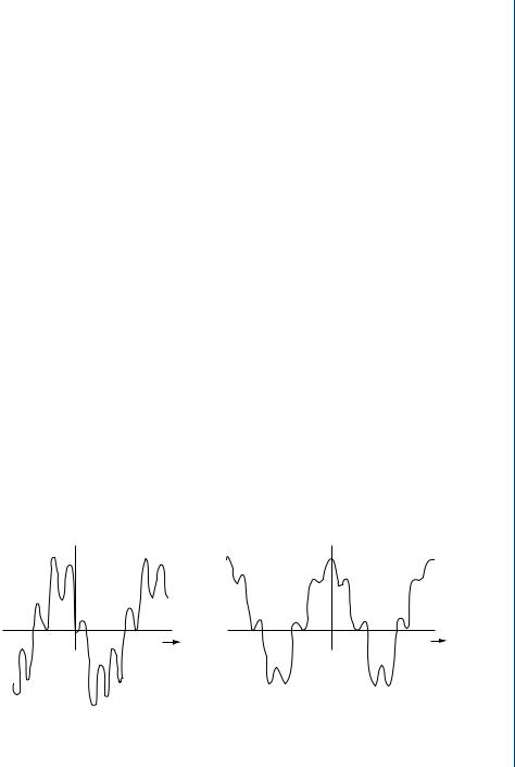
f2(t), their common frequency, ω, and their relative phase angle. When the two signals being cross-correlated share a number of common frequencies, each gives a corresponding contribution to the cross-correlation function as shown in Fig. 17.3. Since it retains information about the relative phases of common frequency components in two signals, the cross-correlation function, unlike the autocorrelation function, is not normally an even function of τ (4).

From the previous discussions, it can be seen that the autocorrelation and crosscorrelation functions provide all analytical means, which may evaluate the magnitude

TRANSFER FUNCTION VIA SPECTRAL ANALYSIS 199

FIGURE 17.3: Cross-correlation function. Trace (b) is the cross-spectral estimate of the two

traces in (a). The bottom trace in (a) is the time shifted upper trace

and phase of a system’s time response. The next step is to look at the equivalents of these functions in the frequency domain where computation will be simplified.

17.5 SPECTRAL DENSITY FUNCTIONS

Spectral density functions can be derived in several ways. One method takes the direct Fourier transform of previously calculated autocorrelation and cross-correlation functions to yield the two-sided spectral density functions given in (17.6).

These integrals always exist for finite intervals. The quantities Sx x ( f ) and Sy y ( f ) are the autospectral density functions of signals x(t) and y (t) respectively, and Sx y ( f ) is the cross-spectral density function between x(y ) and y (t). These quantities are related