

Signal Processing of Random Physiological Signals - Charles S. Lessard
.pdf111
C H A P T E R 1 1
Digital Filters
This chapter will review the concept of filters before presenting an overview of digital filters. It is not the intent of the chapter to enable the reader to write digital filter programs, but rather to present the engineer with the ability to use application software with filters and to choose the proper filter for specific biomedical applications. Let us start with the basic question, “What are Filters?” By definition, “Filters are circuits that pass the signals of certain frequencies and attenuate those of other frequencies.”
11.1CLASSIFICATION OF FILTERS
The most common classification or types of filters are as follows:
1.Low-pass: pass low frequencies; block high frequencies
2.High-pass: pass high frequencies; block low frequencies
3.Band-pass: pass a band of frequencies
4.Band-reject: attenuate a band of frequencies
5.All-pass filter: used for phase shifting
In addition filters are also categorized as follows:
1.Butterworth
a.Low-pass filter
b.High-pass filter, etc.

112SIGNAL PROCESSING OF RANDOM PHYSIOLOGICAL SIGNALS
2.Chevbychev
a.Low-pass filter
b.High-pass filter, etc.
Other classifications that are also used in conjunction with the previous classification are
1.Voltage Controlled Voltage Source (VCVS),
2.Bi Quad,
3.Elliptical, and
4.Digital.
The most common digital filters fall into one of two classes:
1.Finite Impulse Response (FIR) and
2.Infinite Impulse Response (IIR)
Filters are generally described mathematically by their “Transfer Function” in the Time domain as differential equations, or in the Frequency domain as the ratio of two polynomials in “s-domain” or as j ω in radians. The order of a filter is defined by the degree of the denominator. The higher the order, the closer the filter approaches the ideal filter; however, the tradeoff an engineer must make is that higher order filters require more complex hardware, and consequently, are more expensive (costly).
11.1.1Low-Pass Butterworth Filter
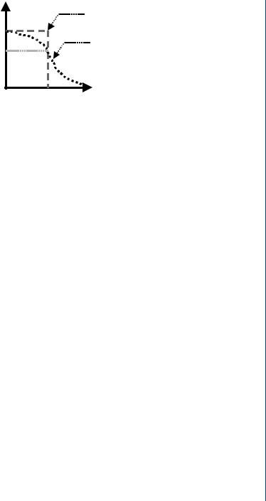
In many applications, the most common low-pass filter used is referred to as an “All-Pole Filter,” which implies that the filter contained “All poles” and “No zeros” in the s-plane. In addition, the all pole, low-pass filter may be called a “Butterworth filter,” which means that the filter has an “over damped” response. Figure 11.1 shows the ideal response of a low-pass Butterworth filter with its cutoff frequency at ωc and the practical response for the same cutoff frequency. It should be noted that the low-pass Butterworth filter
DIGITAL FILTERS 113
H(s) |
Ideal low-pass f ilter |
|
A0
Practical low-pass f ilter
0.707 A0
w
wc
FIGURE 11.1: Butterworth low-pass characteristic transfer function response curves. The ideal
low-pass filter is shown as the red trace, and the normal practical response trace is shown in black
magnitude monotonically decreases as frequency increases in both the band-pass and band-stop regions. The flattest magnitude of the filter is in the vicinity of ω = 0, or DC, with its greatest error about the cutoff frequency.
The “Transfer Function” or describing equation for the Butterworth low-pass filter is given by (11.1) for the s-domain and rewritten in (11.2) in terms of frequency.
H(s ) = |
|
K |
= |
Alp |
|
|
|
(11.1) |
||||||||
s + 1 |
|
s + j ω |
|
|
|
|||||||||||
H( j ω) = |
|
|
Alp |
|
|
|
(11.2) |
|||||||||
|
|
|
|
|
|
|
|
|||||||||
|
|
2 |
|
|
|
|||||||||||
|
|
|
|
|
|
|
|
1 + |
ω |
|
|
|
|
|||
|
|
|
|
|
|
|
|
ωc |
|
|
|
|
|
|||
where Alp = Low-pass gain, and |
|
ω |
|
|
|
|
|
|
|
|
|
|||||
|
|
= ωn |
|
|
|
|
|
|
|
|
|
|||||
ωc |
|
|
|
|
|
|
|
|
|
|||||||
The second-order transfer function for a low-pass Butterworth filter is given by |
||||||||||||||||
(11.3): |
|
|
|
|
|
|
|
|
|
|
|
|
|
|
|
|
H(s ) = |
|
|
|
Alpωn2 |
|
|
|
|
||||||||
s 2 + 2ζ ωns + bωn2 |
|
(11.3) |
||||||||||||||
where |
bωc2 = |
|
|
|
1 |
|
|
|
|
1 |
|
|||||
|
|
|
|
|
= |
|
|
|||||||||
R1 R2C1C2 |
T1T2 |
|
||||||||||||||
11.1.2Chebyshev low-pass Filter
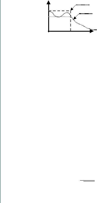
The Chebyshev low-pass filter has an underdamped response, meaning that a filter of second order or higher order may oscillate and become unstable if the gain is too high
114 SIGNAL PROCESSING OF RANDOM PHYSIOLOGICAL SIGNALS
A
A0
Ripple width
Ideal low-pass filter
|
Practical low-pass filter |
wc |
w |
FIGURE 11.2: Chebyshev low-pass characteristic transfer function response curves. The ideal low-pass filter is shown as the dash-line trace, and the normal practical response trace is shown as the dotted-line trace. Note the ripple in the band-pass region
or the input is large. Hence, the term that the “filter rings,” meaning it oscillates during it damping phase. The Chebyshev filter response best approaches the “Ideal filter” and is most accurate near the filter cutoff frequency, but at the expense of having ripples in the band-pass region. It should be noted that the filter is monotonic in the stop-band as is the Butterworth low-pass filter. Figure 11.2 shows the ideal response of a Chebyshev low-pass filter with its cutoff frequency at ωc and the practical response for the same cutoff frequency.
The “Transfer Function” or describing equation for the Butterworth low-pass filter is given by (11.4) in terms of frequency.
H( j ω) = |
|
Alp |
|
|
(11.4) |
|
|
|
|
||
|
1 + ε2Cn2 |
|
|
||
|
|
ω |
|
||
|
|
ωc |
|||
where ε is a constant, and Cn is the Chebyshev polynomial, Cn(x) = cos[n cos −1(x)] The ripple factor is calculated from (11.5).
1 |
|
RW = 1 − √1 + ε2 |
(11.5) |
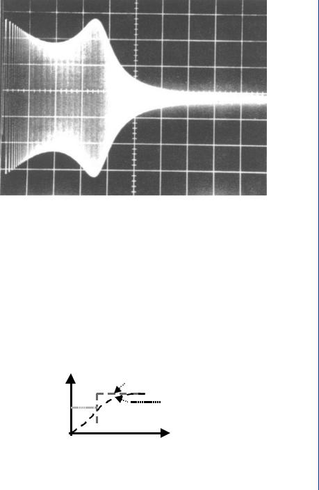
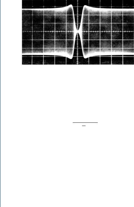
Figure 11.3 shows the response of a third-order Chebyshev Voltage Controlled Voltage Source (VCVS) low-pass filter.
DIGITAL FILTERS 115
FIGURE 11.3: Chebyshev low-pass filter. Response of a third-order Chebyshev as shown by an
oscilloscope
11.1.3Butterworth High-Pass Filter
High-pass filters are designed to pass high frequencies and block low frequencies. As shown in Fig. 11.4, the Butterworth high-pass Filter magnitude monotonically decreases as frequency decreases, with the flattest magnitude in the high frequencies and the greatest error about the cutoff frequency.
H(s)


 Ideal high-pass
A0
Practical high-pass
0.707 A0
 w wc
w wc
FIGURE 11.4: Butterworth high-pass transfer function characteristic curves. The ideal highpass filter is shown as the square trace, and the normal practical response trace is shown in dashed-line black

116 SIGNAL PROCESSING OF RANDOM PHYSIOLOGICAL SIGNALS
The “Transfer Function” or describing equation for the first-order Butterworth high-pass filter is given by (11.6) for the s-domain and rewritten in (11.7) in terms of frequency. It should be noted that the high-pass filter is not an “All Pole Filter,” since the equations show a zero or an s in the numerator of the equations. Hence, in the s-plane a zero exists at the origin, s = 0.
H(s ) = |
K s |
= |
Ahps |
(11.6) |
|||
ωc |
s |
|
ωc |
||||
|
s + b |
|
+ b |
|
|||
H( j ω) = |
|
Ahps |
|
|
(11.7) |
||
|
1 |
|
|
||||
|
s |
+ R1C |
|
||||
where Ahp = high-pass gain.
11.1.42nd-Order Butterworth High-Pass Filter
The transfer function for a second-order Butterworth high-pass filter is given by (11.8):
H(s ) = |
|
|
Ahpbs 2 |
(11.8) |
|||
|
2 |
a |
ωc2 |
||||
|
s |
|
+ b |
ωcs + |
|
|
|
|
|
b |
|
||||
11.1.5Band-Pass Filters
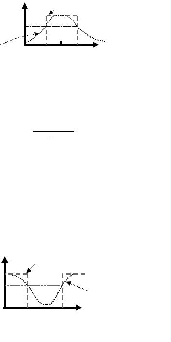
Band-pass filters may be of the Butterworth or of the Chebyshev class. Band-pass filters are designed to pass a band of frequencies of bandwidth, B, with the center of the band around a center frequency (ω0 rad/sec) or f0 = ω0/2π Hz. Band-pass filter must designate two cutoff frequencies: a lower cutoff, ωL, and an upper cutoff, ωU.
The frequencies that are passed by the filter are those for which the transfer function, H (s), gain is greater than or equal to 0.707A0 as shown in Fig. 11.5.
11.1.5.1 Quality Factor
Quality Factor (Q) is a measure of narrowness of the band-pass filter. By definition, the quality factor, Q, is the ratio of the center frequency, ω0, to the bandwidth, B = ωU − ω L in radians per second; hence, the ratio may be expressed as Q = ω0/ B or Q = f0/ B. If the quality factor, Q, is greater than 10, the band-pass region is considered to be narrow. The gain of the band-pass filter is the magnitude at the center frequency. The transfer function for the band-pass filter is given by (11.9). Band-pass filters must be of second
DIGITAL FILTERS 117
Ideal Band-pass
A0 |
|
|
|
0.707 A0 |
|
|
|
|
wL |
w0 |
w |
Practical filter |
wU |
FIGURE 11.5: Band-pass filter transfer function characteristic curves. The ideal band-pass filter
is shown as the dashed-line trace, and the normal practical response trace is shown as dotted-line
trace
or higher order, since the filters require two slopes (high and low). Note that band-pass filters are not All-Pole filters, since the equation shows a zero in the numerator.
ABPω0s |
(11.9) |
H(s ) = s 2 + ωQ0 s + ω02 |
11.1.6Band-Reject or “Notch” Filters
Band-reject filters may be of the Butterworth or of the Chebyshev class. Band-reject filters are designed to attenuate or reject a band of frequencies of bandwidth, B, with the center of the band around a center frequency (ω0 rad/sec) or f0 = ω0/2π Hz. As with the band-pass filter, it is necessary to designate the two cutoff frequencies for a band-reject filter; the lower cutoff, ωL, and the upper cutoff, ωU. The frequencies that are passed by the filter are those for which the transfer function, H (s), gain is greater than or equal to 0.707A0 as shown in Fig. 11.6.
H(s) |
Ideal Notch |
|
|
A0 |
|
|
|
0.707 A0 |
|
|
|
|
|
|
Practical filter |
|
wL |
w0 |
wU |
FIGURE 11.6: Band-reject filter transfer function characteristic curves. The ideal band-reject or notch filter is shown as the dashed-line trace, and the normal practical response trace is shown in dotted-line trace
118 SIGNAL PROCESSING OF RANDOM PHYSIOLOGICAL SIGNALS
FIGURE 11.7: Chebyshev band-reject filter. Response of a fourth-order Chebyshev notch filter
as shown by on an oscilloscope
The transfer function for the band-reject filter is given by (11.10). Band-reject filters must be of second or higher order, since the filters require two slopes (high and low). Note that band-reject filters are not All-Pole filters, since the equation shows a pair of zeros in the numerator (s 2).
ABR(s 2 + ω02) |
|
H(s ) = s 2 + ωQ0 s + ω02 |
(11.10) |
Figure 11.7 shows the response of a fourth-order Chebyshev band-reject (notch) filter. It should be noted that the maximum attenuation of the band-reject filter is the magnitude at the center frequency, ω0.
11.2DIGITAL FILTERS
11.2.1Classification of Digital Filters
The classification of digital filters is similar to the classification of analog filters
1.Chebyshev filters: low-pass or high-pass (Figs. 11.8 and 11.9)
a.Underdamped, can oscillate
b.Ripple factor
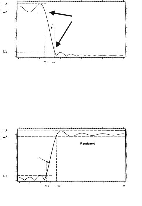
Magnitude
1.0
0.8 Passband
0.6
0.4
0.2
0
0
DIGITAL FILTERS 119
Note
End of pass-band
Transition Start of stop-band band
Stopband
p
Frequency (rad)
FIGURE 11.8: Low-pass filter. In specifying a digital filter, the end of pass-band and the stopband parameters must be designated
2.Butterworth filters
a.Overdamped
b.Monotonic increasing or decreasing function
3.Elliptical filters
Magnitude
1.0
0.8 |
Passband |
0.6Transition
band
0.4
0.2Stopband
0
0 |
p |
|
Frequency (rad)
FIGURE 11.9: High-pass filter. In specifying a digital filter, the end of pass-band and the stopband parameters must be designated. Note the stop-band, the transition band, and the pass-band
120SIGNAL PROCESSING OF RANDOM PHYSIOLOGICAL SIGNALS
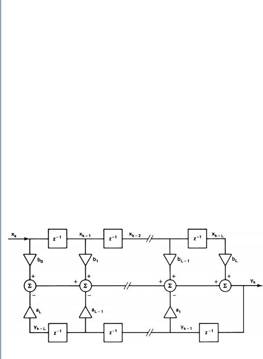
11.2.2Infinite Impulse Response (IIR) Digital Filters
The Pole-zero transfer function of an Lth-order direct form Infinite Impulse Response Filter (IIR-filter) has the z-transform transfer function described by (11.11).
H (z) = |
B (z) |
= |
bo + b1−Z1 + · · · + b−LZL |
(11.11) |
||||
A (z) |
|
|
1 + a |
−1 |
−L |
|||
|
|
|
|
|
1Z |
+ · · · + aLZ |
|
|
where the zs are the “z-transformation.”
General characteristics of the infinite impulse response filters are as follows:
a.Very sharp cutoff
b.Narrow transition band
c.Low-order structure
d.Low-processing time
There are several designs that can be used to implement (11.11), such as the direct, parallel, or cascade design. The “Direct” design is shown in Fig. 11.10, whereas a “Symmetric Lattice” of the IIR design is shown in Fig. 11.11.
x |
k |
|
|
|
|
|
|
|
|
|
|
|
|
|
|
|
xk—1 |
|
|
|
|
|
|
|
|
xk—2 |
|
|
|
|
|
|
|
|
|
|
|
|
|
|
|
|
xk—L |
|
|
|
|
|
|
|||||||
|
|
|
|
|
|
|
|
|
|
|
|
|
|
|
|
|
|
|
|
|
|
|
|
|
|
|
|
|
|
|
|
|
|
|
|
|
|
|
|
|
|
|
||||||||||||||
|
|
|
|
|
|
|
|
|
|
z–1 |
|
|
|
|
|
|
|
|
|
z–1 |
|
|
|
|
|
|
|
|
|
|
|
|
|
|
|
z–1 |
|
|
|
|
|
|
||||||||||||||
|
|
|
|
|
|
|
|
|
|
|
|
|
|
|
|
|
|
|
|
|
|
|
|
|
|
|
|
|
|
|
|
|
|
|
|
|
|
|
|
|
|
|
|
|
|
|
|
|
|
|
|
|
||||
|
|
|
|
|
|
|
|
|
|
|
|
|
|
|
|
|
|
|
|
|
|
|
|
|
|
|
|
|
|
|
|
|
|
|
|
|
|
|
|
|
|
|
|
|
|
|
|
|
|
|
|
|
|
|
|
|
|
|
|
|
|
|
|
|
|
|
|
|
|
|
|
|
|
|
|
|
|
|
|
|
|
|
|
|
|
|
|
|
|
|
|
|
|
|
|
|
|
|
|
|
|
|
|
|
|
|
|
|
|
|
|
|
|
|
|
|
|
|
|
|
|
|
|
|
|
|
|
|
|
|
|
|
|
|
|
|
|
|
|
|
|
|
|
|
|
|
|
|
|
|
|
|
|
|
|
|
|
|
|
|
|
|
|
|
|
|
|
|
|
|
|
|
|
|
|
|
|
|
|
|
|
|
|
|
|
|
|
|
|
|
|
|
|
|
|
|
|
|
|
|
|
|
|
|
|
|
|
|
bL—1 |
|
|
|
|
|
|
|
|
|
|
|
bL |
|
|
||||
|
|
|
|
|
|
|
|
b0 |
|
|
|
|
|
|
|
|
|
|
|
b1 |
|
|
|
|
|
|
|
|
|
|
|
|
|
|||||||||||||||||||||||
|
|
|
|
|
|
|
|
|
|
|
|
|
|
|
|
|
|
|
|
|
|
|
|
|
|
|
|
|
|
|
|
|
|
|
|
|
|
|
|
|
|
|
|
|
|
|
|
|
|
|
|
|
|
|
|
|
|
|
|
|
|
|
|
|
|
|
|
|
|
|
|
|
|
|
|
|
|
|
|
|
|
|
|
|
|
|
|
|
|
|
|
|
|
|
|
|
|
|
|
|
|
|
|
|
|
|
|
|
|
|
|
||
|
|
|
|
+ |
|
|
|
|
|
|
|
|
|
|
|
|
|
|
|
|
|
|
|
|
|
|
|
|||||||||||||||||||||||||||||
|
|
|
|
|
|
|
|
|
|
|
|
|
+ |
|
|
|
|
|
|
|
|
|
|
|
|
|
|
|
|
|
|
|
|
|
|
+ |
|
|
|
|||||||||||||||||
|
|
|
|
|
|
|
|
|
|
|
|
|
|
|
|
|
|
|
|
|
|
|
|
+ |
|
|
|
|
|
|
|
|
|
|
|
|
|
|
|
|
|
|||||||||||||||
|
|
|
|
|
|
|
|
|
|
|
|
|
|
|
|
|
|
|
|
|
|
|
|
|
|
|
|
|
|
|
|
|
+ |
|
|
|
|
|
yk |
|||||||||||||||||
|
|
|
|
|
|
|
|
|
|
|
|
|
|
|
+ |
|
|
|
|
|
|
|
|
|
|
|
|
|
|
|
|
|
|
|
|
|
|
|
|
|
|
|
|
|
|
|
|
|
|
|
|
|
||||
|
|
|
|
|
|
|
|
|
|
|
|
|
|
|
|
|
|
|
|
|
|
|
|
|
|
|
|
|
+ |
|
|
|
|
|
|
|
|
|
|
|
|
|
|
|
|
|
|
|
|
|
||||||
|
|
|
|
|
|
|
|
|
|
|
|
|
|
|
|
|
|
|
|
|
|
|
|
|
|
|
|
|
|
|||||||||||||||||||||||||||
|
|
|
|
|
|
|
|
|
|
|
|
|
|
|
|
|
|
|
|
|
|
|
|
|
|
|
|
|
|
|
|
|
|
|
|
|
|
|
|
|
|
|
|
|
|
|||||||||||
|
|
|
|
|
|
|
|
|
|
|
|
|
|
|
|
|
|
|
|
|
|
|
|
|
||||||||||||||||||||||||||||||||
|
|
|
|
|
|
|
|
|
|
|
|
|
|
|
|
|
|
|
|
|
|
|
|
|
|
|
|
|
|
|
|
|
|
|
|
|
|
|
|
|
|
|
|
|
|
|
|
|
|
|
|
|
|
|
|
|
|
|
|
|
|
|
|
|
|
|
|
|
|
|
|
|
|
|
|
|
|
|
|
|
|
|
|
|
|
|
|
|
|
|
|
|
|
|
|
|
|
|
|
|
|
|
|
|
|
|
|
|
|
|
|
|
|
|
|
|
|
|
|
|
|
|
|
|
|
|
|
|
|
|
|
|
|
|
|
|
|
|
|
|
|
|
|
|
|
|
|
|
|
|
|
|
|
|
|
|
|
|
|
|
|
|
||||||||
|
|
|
|
|
|
– |
– |
|
|
|
|
|
|
|
|
|
– |
|
|
|
|
|
|
|
|
|
|
|
|
|
||||||||||||||||||||||||||
|
|
|
|
|
|
|
|
|
|
|
|
|
|
|
|
|
|
|
|
|
|
|
|
|
|
|
|
|
|
|
|
|
|
|
|
|
|
|
|
|
|
|
|
|
|
|
||||||||||
|
|
|
|
|
|
|
aL |
|
|
|
|
|
|
|
|
|
|
|
aL—1 |
|
|
|
|
|
|
|
|
|
|
|
a1 |
|
|
|
|
|
|
|
|
|
|
|
|
|
|
|||||||||||
|
|
|
|
|
|
|
|
|
|
|
|
|
|
|
|
|
|
|
|
|
|
|
|
|
|
|
|
|
|
|
|
|
|
|
|
|
|
|
|
|
|
|
|
|
|
|
|
|
|
|
|
|
|
|
|
|
|
|
|
|
|
|
|
|
|
|
|
|
|
|
|
|
|
|
|
|
|
|
|
|
|
|
|
|
|
|
|
|
|
|
|
|
|
|
|
|
|
|
|
|
|
|
|
|
|
|
|||||||
|
|
|
|
|
|
yk—L |
|
|
|
|
|
|
|
|
|
|
|
|
|
|
|
|
|
|
|
|
|
|
|
|
|
|
|
|
|
yk—1 |
|
|
|
|
|
|
|
|
|
|
|
|
|
|||||||
|
|
|
|
|
|
|
|
|
|
|
|
|
|
|
|
|
|
|
|
|
|
|
|
|
|
|
|
|
|
|
|
|
|
|
|
|
|
|
|
|
|
|
|
|
|
|||||||||||
|
|
|
|
|
|
|
z–1 |
|
|
|
|
|
|
|
|
|
|
|
|
|
|
z–1 |
|
|
|
|
|
|
|
|
|
|
|
|
|
z–1 |
|
|
|
|
|
|
|
|
|
|||||||||||
|
|
|
|
|
|
|
|
|
|
|
|
|
|
|
|
|
|
|
|
|
|
|
|
|
|
|
|
|
|
|
|
|
|
|
|
|
|
|
|
|
|
|
|
|
|
|
|
|
|
|||||||
|
|
|
|
|
|
|
|
|
|
|
|
|
|
|
|
|
|
|
|
|
|
|
|
|
|
|
|
|
|
|
|
|
|
|
|
|
|
|
|
|
|
|
|
|
|
|
|
|
|
|
|
|
|
|
|
|
FIGURE 11.10: Direct-form IIR digital filter. Note the numerator coefficients are the bL terms and the denominator coefficients are the aL terms