Don’t forget to define GLEW_STATIC either using this preprocessor directive or by adding the -DGLEW_STATIC directive to your compiler command-line parameters or project settings.

If you prefer to dynamically link with GLEW, leave out the define and link with glew32.lib instead of glew32s.lib on Windows. Don’t forget to include glew32.dll or libGLEW.so with your executable!

Now all that’s left is calling glewInit() after the creation of your window and OpenGL context. The glewExperimental line is necessary to force GLEW to use a modern OpenGL method for checking if a function is available.

glewExperimental = GL_TRUE; glewInit();

Make sure that you’ve set up your project correctly by calling the glGenBuffers function, which was loaded by GLEW for you!

GLuint vertexBuffer; glGenBuffers(1, &vertexBuffer);

printf("%u\n", vertexBuffer);

Your program should compile and run without issues and display the number 1 in your console. If you need more help with using GLEW, you can refer to the website or ask in the comments.

Now that we’re past all of the configuration and initialization work, I’d advise you to make a copy of your current project so that you won’t have to write all of the boilerplate code again when starting a new project.

Now, let’s get to drawing things!

Drawing

The graphics pipeline

By learning OpenGL, you’ve decided that you want to do all of the hard work yourself. That inevitably means that you’ll be thrown in the deep, but once you understand the essentials, you’ll see that doing things the hard way doesn’t have to be so di cult after all. To top that all, the exercises at the end of this chapter will show you the sheer amount of control you have over the rendering process by doing things the modern way!

The graphics pipeline covers all of the steps that follow each other up on processing the input data to get to the final output image. I’ll explain these steps with help of the following illustration.

18

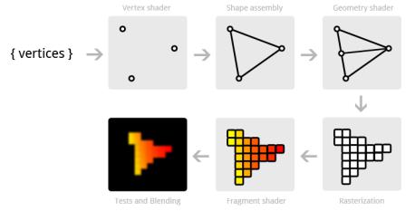
Figure 4:

It all begins with the vertices, these are the points from which shapes like triangles will later be constructed. Each of these points is stored with certain attributes and it’s up to you to decide what kind of attributes you want to store. Commonly used attributes are 3D position in the world and texture coordinates.

The vertex shader is a small program running on your graphics card that processes every one of these input vertices individually. This is where the perspective transformation takes place, which projects vertices with a 3D world position onto your 2D screen! It also passes important attributes like color and texture coordinates further down the pipeline.

After the input vertices have been transformed, the graphics card will form triangles, lines or points out of them. These shapes are called primitives because they form the basis of more complex shapes. There are some additional drawing modes to choose from, like triangle strips and line strips. These reduce the number of vertices you need to pass if you want to create objects where each next primitive is connected to the last one, like a continuous line consisting of several segments.

The following step, the geometry shader, is completely optional and was only recently introduced. Unlike the vertex shader, the geometry shader can output more data than comes in. It takes the primitives from the shape assembly stage as input and can either pass a primitive through down to the rest of the pipeline, modify it first, completely discard it or even replace it with other primitive(s). Since the communication between the GPU and the rest of the PC is relatively slow, this stage can help you reduce the amount of data that needs to be transferred. With a voxel game for example, you could pass vertices as point vertices, along with an attribute for their world position, color and material and the actual cubes can be produced in the geometry shader with a

19

point as input!

After the final list of shapes is composed and converted to screen coordinates, the rasterizer turns the visible parts of the shapes into pixel-sized fragments. The vertex attributes coming from the vertex shader or geometry shader are interpolated and passed as input to the fragment shader for each fragment. As you can see in the image, the colors are smoothly interpolated over the fragments that make up the triangle, even though only 3 points were specified.

The fragment shader processes each individual fragment along with its interpolated attributes and should output the final color. This is usually done by sampling from a texture using the interpolated texture coordinate vertex attributes or simply outputting a color. In more advanced scenarios, there could also be calculations related to lighting and shadowing and special e ects in this program. The shader also has the ability to discard certain fragments, which means that a shape will be see-through there.

Finally, the end result is composed from all these shape fragments by blending them together and performing depth and stencil testing. All you need to know about these last two right now, is that they allow you to use additional rules to throw away certain fragments and let others pass. For example, if one triangle is obscured by another triangle, the fragment of the closer triangle should end up on the screen.

Now that you know how your graphics card turns an array of vertices into an image on the screen, let’s get to work!

Vertex input

The first thing you have to decide on is what data the graphics card is going to need to draw your scene correctly. As mentioned above, this data comes in the form of vertex attributes. You’re free to come up with any kind of attribute you want, but it all inevitably begins with the world position. Whether you’re doing 2D graphics or 3D graphics, this is the attribute that will determine where the objects and shapes end up on your screen in the end.

Device coordinates

When your vertices have been processed by the pipeline outlined above, their coordinates will have been transformed into device coordinates. Device X and Y coordinates are mapped to the screen between -1 and 1.

20

Just like a graph, the center has coordinates (0,0) and the y axis is positive above the center. This seems unnatural because graphics applications usually have (0,0) in the top-left corner and (width,height) in the bottom-right corner, but it’s an excellent way to simplify 3D calculations and to stay resolution independent.

The triangle above consists of 3 vertices positioned at (0,0.5), (0.5,-0.5) and (-0.5,-0.5) in clockwise order. It is clear that the only variation between the vertices here is the position, so that’s the only attribute we need. Since we’re passing the device coordinates directly, an X and Y coordinate su ces for the position.

OpenGL expects you to send all of your vertices in a single array, which may be confusing at first. To understand the format of this array, let’s see what it would look like for our triangle.

float vertices[] = {

0.0f, 0.5f, // Vertex 1 (X, Y)

21

0.5f, -0.5f, // Vertex 2 (X, Y) -0.5f, -0.5f // Vertex 3 (X, Y)

};

As you can see, this array should simply be a list of all vertices with their attributes packed together. The order in which the attributes appear doesn’t matter, as long as it’s the same for each vertex. The order of the vertices doesn’t have to be sequential (i.e. the order in which shapes are formed), but this requires us to provide extra data in the form of an element bu er. This will be discussed at the end of this chapter as it would just complicate things for now.

The next step is to upload this vertex data to the graphics card. This is important because the memory on your graphics card is much faster and you won’t have to send the data again every time your scene needs to be rendered (about 60 times per second).

This is done by creating a Vertex Bu er Object (VBO):

GLuint vbo;

glGenBuffers(1, &vbo); // Generate 1 buffer

The memory is managed by OpenGL, so instead of a pointer you get a positive number as a reference to it. GLuint is simply a cross-platform substitute for unsigned int, just like GLint is one for int. You will need this number to make the VBO active and to destroy it when you’re done with it.

To upload the actual data to it you first have to make it the active object by calling glBindBuffer:

glBindBuffer(GL_ARRAY_BUFFER, vbo);

As hinted by the GL_ARRAY_BUFFER enum value there are other types of bu ers, but they are not important right now. This statement makes the VBO we just created the active array buffer. Now that it’s active we can copy the vertex data to it.

glBufferData(GL_ARRAY_BUFFER, sizeof(vertices), vertices, GL_STATIC_DRAW);

Notice that this function doesn’t refer to the id of our VBO, but instead to the active array bu er. The second parameter specifies the size in bytes. The final parameter is very important and its value depends on the usage of the vertex data. I’ll outline the ones related to drawing here:

•GL_STATIC_DRAW: The vertex data will be uploaded once and drawn many times (e.g. the world).

•GL_DYNAMIC_DRAW: The vertex data will be created once, changed from time to time, but drawn many times more than that.

•GL_STREAM_DRAW: The vertex data will be uploaded once and drawn once.

This usage value will determine in what kind of memory the data is stored on your graphics card for the highest e ciency. For example, VBOs with

22