found as the d dominant left singular vectors of Γ(X) R M×2N (direct data approach) or Γ(X)Γ(X)H RM×M (covariance approach). This principle is applied to formulate a new version of ESPRIT called the unitary ESPRIT, which is described next.

5.5 Unitary ESPRIT in Element Space

Unitary ESPRIT is applicable to centro-symmetric array configurations and it includes forward-backward averaging [3]. The complex-valued factorizations like SVD or EVD are transformed into real-valued factorizations. The element space implementation of unitary ESPRIT is discussed in detail in this section. Another approach, the unitary ESPRIT in DFT beamspace, which focuses on a particular DOA sector of interest with the reduced computational complexity, will be described later.

5.5.1One-Dimensional Unitary ESPRIT in Element Space

Unitary ESPRIT performs the computations in real instead of complex numbers from the beginning to the end of the algorithm. The concepts explained with centro-symmetric arrays in Section 3.3 and the fundamental theorem reviewed in the previous section are employed to achieve this real-valued estimation. In this section, each step of the algorithm, that is, estimation of the signal subspace estimation, the solution of the invariance equation, and the computation of DOAs, will be presented with real-valued calculations.

5.5.1.1 Real-Valued Subspace Estimation

Consider a uniform linear array (ULA) with maximum overlap. Assume the signal and data model discussed in Chapter 2. Suppose that the real-valued data matrix from the transformation Γ(X) and its real-valued covariance matrix Rxx are obtained using unitary transformations as discussed in the previous section. Also, this unitary transformation includes forward-backward averaging. Let the d dominant left singular vectors of Γ(X) R M×2N (direct data approach) or the d dominant eigenvectors of Γ(X)Γ(X)H R M×M (covariance approach) be Es R M×d. Then,

contains a basis for the estimated signal subspace. More specifically, the columns of Us in (5.29) contain d dominant left singular vectors of the extended data matrix Z or d dominant eigenvectors of ZZH. From now, we refer to the subspace spanned by Es as the real-valued signal subspace. The real-valued and complex-valued subspaces are related by (5.29). In the next step, the real-valued invariance equation is formulated.

5.5.1.2 Real-Valued Invariance Equation

In this section, the approach to transforming the complex-valued invariance equation of a uniform linear array with a maximum overlap into a real-valued equation is presented.

Consider the complex-valued invariance equation (5.11) rewritten here for ready reference.

Denote b(μi) as the real-valued transformed steering vector; then by Theorem 5.1, it can be obtained as:

where Qm and QM are unitary and left Π-real matrices. Since QM is unitary, it follows that

Premultiplying both sides by Q mH gives the following invariance relationship

By definition of tangent function, the above invariance relationship satisfied by b(μi) can be expressed finally in real-valued quantities [6]:

For d impinging signals, we define the real-valued transformed steering matrix of size M × d as

98 Introduction to Direction-of-Arrival Estimation

with = diag{ω1, ω2, …, ωi, …, ωd} being the eigenvalues of ϒ. The

A summary of computational steps of one-dimensional unitary ESPRIT is tabulated in Table 5.2 [1].

In the next section, unitary ESPRIT is extended to two-dimensional arrays for estimating the DOA in both azimuthal and elevational angles.

5.5.2Two-Dimensional Unitary ESPRIT in Element Space

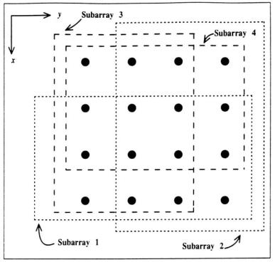
A fundamental restriction of one dimensional array is that they can only estimate a single direction parameter. For a joint azimuthal and elevation angle estimation, a two-dimensional array is required. Consider a uniform rectangular array (URA) of size M = Mx My in the x-y plane where the interelement spacing in the x and y directions are x and y, respectively. In addition, assume that the centro-symmetric arrays also exhibits a dual invariance, that is, two identical subarrays ofmx elements are displaced by x along the x-axis and another pair of identical subarrays, each

Table 5.2

Summary of One-Dimensional Unitary ESPRIT Algorithm

1. Real-Valued Subspace Estimation: Compute Es

as the d dominant left singular vectors of Γs(X) (square-root approach) or as the d dominant eigenvectors of Γs(X)Γs(X)H (covariance approach)

2. Real-Valued Invariance Equation: Solve the following equation for ϒ

K1E s ϒ ≈ K 2E s

by means of LS or TLS

3. DOA Estimation: Calculate the eigenvalues of the resulting complex-valued solution ϒ = TΩT−1 with Ω = diag{ω1, ω2 , ωi , , ωd }

which satisfies the centro-symmetric condition. The approach is to decompose the two-dimensional URA problem into two independent one-dimensional problems [1, 8]. Then, we can estimate the spatial frequencies with respect to each array separately. The spatial frequencies μi in the x direction and νi in the y direction are scaled versions of the corresponding direction cosines, namely,

As described in Section 2.3.2, the DOAs can be found through the following relationship:

φi = arg(ui + jvi ) and θi = arcsin(ui + jvi )

Like the one-dimensional unitary ESPRIT, to find these values, the signal subspace and the invariance equation need to be estimated.

5.5.2.1 Real-Valued Signal Subspace Estimation

As the first step, the real-valued signal subspace is obtained from the data matrix. This is obtained identically as the case for the one-dimensional ULA except that the data matrix employed here consists of stacked data from a uniform rectangular array. The real-valued data matrix from the transformation Γ(X) and the real-valued covariance matrix Rxx are obtained using the unitary transformations as discussed in Section 5.5.1. It was observed that this unitary transformation also includes for- ward-backward averaging. Let the d dominant left singular vectors of

contains a basis for the estimated signal subspace. The columns of Us in (5.51) contain d dominant left singular vectors of the extended data matrix Z or d dominant eigenvectors of ZZH. The real-valued and com- plex-valued subspaces are related through (5.51). As the next step two

invariance equations are formulated, which are later transformed into real-valued.

5.5.2.2 Real-Valued Invariance Equation

As the URA is subdivided into two pairs of subarrays with maximum overlap, two pairs of selection matrices are defined similar to (5.9): one-dimensional selection matrices for the uniform linear arrays in the x direction are

Similarly, the one-dimensional selection matrices for the ULAs in the y direction are given by

The array manifold matrices satisfy the invariance relation and can be expressed

Now applying the vec{•} operator to (5.54) and using the property in the Appendix, Section A.1,

The two-dimensional selection matrices of the URA (corresponding to maximum overlap) can be obtained as the following Kronecker products [1, 7]:

These real-valued selection matrices are thus used to obtain the real-valued invariance equation.

5.5.2.3 DOA Estimation

Let the columns of Es span the estimated real-valued signal subspace, which is the dominant subspace of Γ(X) as discussed in Section 5.4. As before, Es may be computed as the d largest singular vectors of Γs(X) (direct data approach) or the d dominant eigenvectors of Γs(X)Γs(X)H (covariance approach). Es and B span the same signal subspace. Therefore, there is a nonsingular matrix TA of size d × d such that

Substitution of the above relation into (5.60) gives two real-valued invariance equations:

where the real-valued matrices can be expressed as

contain the desired spatial frequency (DOA) information.

As in the one-dimensional case, the two real-valued invariance equations in (5.63) can be solved independently by LS or TLS. However, the real-valued eigenvalues of the solutionϒ μ andϒ v to the above invariance equations are given by tan(μi /2) and tan(νi /2), respectively. If the eigenvalues of these matrices are calculated independently, it is very

difficult to pair the resulting two distinct estimates of the frequency estimates (i.e., the elevation angle pair of azimuthal angle). To overcome this problem of pairing, an automatic pairing scheme is incorporated in the two-dimensional unitary ESPRIT [9].

5.5.2.4 Automatic Pairing of Spatial Frequency Estimates

The real-valued matrices ϒ μ and ϒ ν share the same set of eigenvectors. It is possible to choose one real-valued eigenvector matrix T such that ϒ μ = TΩ μ T −1 and ϒ ν = TΩ ν T −1 are real-valued. However, due to

additive noise and the finite number of snapshots N, the real-valued matricesϒ μ andϒ ν do not exactly have the same set of eigenvectors. As a result, obtaining eigenvectors from only one of the matrices will give wrong estimates as this would be a random choice since the information in the other matrix is not being used. Also, ϒ μ and ϒ ν might have some degenerate (multiple) eigenvalues, though they have common set of eigenvectors.

This problem is solved in two-dimensional unitary ESPRIT by “making a complex matrix” ϒ μ + jϒ v [9]. An automatic pairing of the spatial frequency estimates μi and νi can then be obtained by computing the eigenvalues of this matrix as

A summary of computations of two-dimensional unitary ESPRIT is given in Table 5.3 [1].