

66 |
Introduction to Direction-of-Arrival Estimation |
research on a separate class of techniques called model order estimation techniques. Model order or source order estimators are mandatory algorithms that are to be run before the DOA estimation algorithms are executed. This chapter gives a brief introduction to some of these techniques.
4.2 Preprocessing Schemes
The subspace-based DOA estimation algorithms are completely based on the full rank condition of the data covariance matrix Rxx given in (2.20). It is written here again for ready reference.
R |
xx |
= E x(t )x H (t ) |
= AR |
ss |
A H + σ 2 |
I |
M |
(4.1) |
|
|
{ |
} |
|
N |
|
|
|||
The condition of Rxx depends on that of signal covariance matrix Rss. When the d impinging signal wavefronts are not correlated, the signal covariance matrix Rss has full rank d; it is diagonal and nonsingular. Rss becomes nondiagonal and singular when the signals are partially correlated, or when some signals are fully correlated (coherent). For instance, if one of the impinging signal wavefronts is highly correlated or coherent with another, their cross-correlation coefficient has a magnitude of 1 and the rank of Rss is now reduced to d − 1. Therefore, the full rank condition in the previously described DOA algorithms is no longer satisfied (i.e., rank {ARss AH} = d − 1); a DOA algorithm will then fail. In general, if there are P coherent wavefronts, Rss is of rank M − P. In such a case, Rxx does not have d large positive eigenvalues, as it otherwise does when the signals are uncorrelated and Rss is diagonal. This implies that the matrix Rss is likely to have fewer than d large positive eigenvalues, creating errors in the DOA estimation processes.
For instance, assume that two of the impinging signals are coherent; say the first two are coherent, that is, s2(t) = αs1(t), with α being a complex scalar describing the gain and phase relationship between the two coherent signals. Then s(t) is a signal vector given by
s(t ) = [s 1 (t ) αs 1 (t ) s 3 (t ) s d (t )]H |
(4.2) |
and the array steering matrix is given by

Preprocessing Schemes and Model Order Estimation |
67 |
||||||||||||
|
|
|
|
|
|
|
|
|
|
|
|
|
|
A = |
[ |
a(θ |
1 |
) a(θ |
2 |
) |
a(θ |
3 |
) a(θ |
d |
] |
|
|
|
|
|
|
|
) |
(4.3) |
|||||||
With these modified |
|
signals, |
|
the signal |
covariance |
matrix Rss = |
|||||||
E{s(t)sH(t)} is now a d × d singular matrix and no longer nonsingular. The following two errors can be observed:
1.The multiplicity of the smallest eigenvalues of Rxx now is k = M − d + 1 and not k = M − d. This gives an error in estimating the number of signals as d − 1(=M − k) instead of d.
2.Only {θ3, …, θd} can be resolved due to the reduced number of resolvable largest eigenvalues of Rxx.
To deal with the issue of the coherent signal reception, a preprocessing scheme such as forward-backward averaging or spatial smoothing can be applied; they ensure Rss (after being smoothed) to be of full rank and nonsingular even when all the received signals are coherent. In other words, the schemes are used basically to decorrelate the signals before estimating their DOAs [1, 2].
4.2.1Forward-Backward Averaging
Forward-backward (FB) averaging is a popular preprocessing scheme employed in many signal processing applications including radio direction finding. Forward-backward averaging can be implemented if the arrays are centro-symmetric in nature. The basic operation of forward backward averaging relies on the fact that the steering vectors of ULA remains the same, even if their elements are reversed and complex conjugated.
Let ΠM be an M × M exchange matrix. Then for ULA it can be shown that [1]
Π M |
|
(θi ) = e − j ( M −1) μi a(θi ) |
(4.4) |
a |
A backward data covariance matrix Rback can then be constructed from the actual data covariance matrix Rxx as
Rback = Π M |
|
xx Π M |
(4.5) |
R |

68 |
Introduction to Direction-of-Arrival Estimation |
Consider a simple case of two coherent sources impinging on a ULA. The forward-backward averaged data covariance matrix is obtained by averaging the actual (forward) covariance matrix and the backward covariance matrix, that is,
R xxfb = |
1 |
(R xx |
+ R back |
) = |
1 |
(R xx + Π M |
|
xx Π M ) |
|
R |
|||||||||
|
|
||||||||
2 |
|
|
2 |
|
|
|
|||
2 |
{ |
{ |
|
} |
|
M |
|
|
{ |
} |
M } |
|
||||||||
= |
1 |
|
E |
x(t )x H (t ) |
+ Π |
|
E |
|
|
(t ) |
|
H (t ) |
Π |
|
(4.6) |
|||||
|
|
x |
x |
|
||||||||||||||||
= A |
1 |
(R ss + R ss |
H |
)A H + σ n2 I M |
|
|
|
|||||||||||||
|
|
|
|
|
||||||||||||||||
|
|
2 |
|
|
|
|
|
|
|
|
|
|
|
|
|
|
|
|
|
|
with some unitary diagonal matrix |
Cd×d [3]. Comparing (4.6) with |
|||||||||||||||||||
(4.1), the new signal covariance matrix is now given by |
|
|
|
|||||||||||||||||
|
|
|
|
|
R ssfb = |
1 |
(R ss + |
|
H ) |
|
|
(4.7) |
||||||||
|
|
|
|
|
|
R |
ss |
|
|
|||||||||||
|
|
|
|
|
|
|
|
|||||||||||||
|
|
|
|
|
2 |
|
|
|
|
|
|
|
|
|
|
|
|
|
|
|
This new forward backward signal covariance matrix has rank d even if the two signals are coherent; it enables the separation of two coherent or highly correlated signals. A forward backward averaged edition of any covariance based algorithm can thus be obtained by replacing R xx with R xxfb in a DOA algorithm. This technique is sometimes used even
in uncorrelated signal environments to obtain more reliable estimates.
In practice, to compute R xxfb |
with data X CM×N received by an |
|||||||||||||||
array, a new extended data matrix Z is used; it is defined as |
|
|
||||||||||||||
|
|
Z = [X |
Π M XΠ N ] C M × 2N |
|
|
|
(4.8) |
|||||||||
An estimate of R xxfb |
can then be calculated as |
|
|
|
|
|||||||||||
fb |
|
1 |
|
|
H |
|
1 |
(XX |
H |
|
|
|
H |
|
) |
|
= |
|
|
= |
+ Π M XX |
Π M |
|
||||||||||
R xx |
2N |
ZZ |
|
2N |
|
|
(4.9) |
|||||||||
|
|
|
|
|
|
|
|
|
|
|
|
|
|
|||
In Chapter 5, it shall be shown that the forward backward averaging is achieved inherently in a unitary ESPRIT algorithm.
Preprocessing Schemes and Model Order Estimation |
69 |
|
|
4.2.2Spatial Smoothing
In a rich multipath area, we may encounter more than two coherent signals. If this is the case, forward-backward averaging alone is not able to decorrelate the signals. Spatial smoothing is another preprocessing technique that can be used to tackle this problem. In spatial smoothing, the antenna array is divided into a number of smaller overlapping subarrays and the data covariance matrices obtained from each subarray are averaged [1–3]. In this section, spatial smoothing techniques applied to ULA and URA are described. These techniques are later applied with ESPRIT when dealing with coherent signals.
4.2.2.1 One-Dimensional Spatial Smoothing
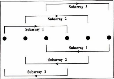
Consider a ULA consisting of M elements as shown in Figure 4.1. Let this ULA be divided into L subarrays, each containing Msub = M − L + 1 elements. There are two types of the divisions shown in Figure 4.1; the upper arrays are called the forward subarrays and the lower arrays are called the backward arrays; either of these types can be used.
Consider the forward or upper subarrays first. The number and size of the subarrays are determined from the number of sources under
Figure 4.1 An example of two different subarrays for one dimensional smoothing. The upper subarrays are called forward subarrays and the lower subarrays are called the backward subarrays.
70 |
Introduction to Direction-of-Arrival Estimation |
consideration. The approach is to form a covariance matrix of each of these subarrays and average them. The formation of the subarrays can be represented mathematically by a selection matrix. For instance, for the lth subarray, the selection matrix is formed here [2, 3]:
( M ) |
= [0 I M sub 0] R |
M sub × M |
, 1 |
≤ l ≤ L |
(4.10) |
Jl |
|
The data matrix corresponding to the lth subarray can then be given
as
( M ) |
X = A |
1Φ |
l −1 |
( M ) |
N, 1≤ l ≤ L |
(4.11) |
X l = Jl |
|
S + Jl |
where A 1 = J(1M ) A. The data covariance matrix of the lth subarray is then obtained as
R l = A |
1Φ |
l −1 |
( M ) |
N, 1≤ l ≤ L |
(4.12) |
|
S + Jl |
The “spatially smoothed data” matrix of the complete array is now obtained from the data matrices of the individual subarrays as
X ss = [J |
( M ) |
X J |
( M ) |
( M ) |
X] C |
M sub × NL |
(4.13) |
1 |
2 |
X J L |
|
Finally, the spatially smoothed data covariance matrix is obtained by taking average of data covariance matrices of the individual subarrays as shown next:
|
|
|
1 |
|
L |
|
|
|
|
|
|
|
|
|
|
|
|
||
R ssxx |
= |
|
∑ R l |
|
|
|
|
|
|
|
|
|
|
|
|||||
|
|
|
|
|
|
|
|
|
|
|
|
|
|||||||
|
|
|
L l =1 |
|
|
|
|
|
|
|
|
|
|
|
|
||||
|
|
1 |
|
|
L |
|
|
|
|
|
|
|
|
|
|
|
|
||
|
= |
∑ Jl( M )R xx Jl( M )T |
|
|
|
|
|
|
|||||||||||
|
|
|
|
|
|
|
(4.14) |
||||||||||||
|
|
L l =1 |
|
|
|
|
|
|
|
|
|
|
|
||||||
|
|
|
|
|
|
1 |
L |
|
l −1 |
|
|
|
l −1 |
|
H |
|
2 |
|
|
|
= A 1 |
∑ Φ |
R ss Φ |
+ σ |
|
||||||||||||||
|
|
|
|
|
A |
1 |
|
I M sub |
|||||||||||
|
|
|
|
|
|||||||||||||||
|
|
|
|
|
|
L l =1 |
|
|
|
|
|
|
|
|
|
|
|
||
|
= A |
1 |
R ss |
A H |
+ |
σ 2I |
M sub |
|
|
|
|
|
|
||||||
|
|
|
|
|
ss |
l |
|
|
|
|
|
|
|
|
|
||||

Preprocessing Schemes and Model Order Estimation |
71 |
|
|
where Rssss = 1 ∑L Φl −1Rss Φl −1 is the newly obtained spatially smoothed
L l =1
signal covariance matrix. Consequently, if there are L coherent wavefronts, the rank of Rss is d − L, but the spatially smoothed signal covariance matrix Rssxx will have the required rank d. Therefore the direc-
tion of arrivals of all d signals can be estimated.
It can be observed from (4.13) that the number of available snapshots is extended from N to NL, whereas the effective aperture of the array is reduced from M to Msub. This is the price for the smoothing. Conventionally, if there are d signals, the minimum number of elements required is M = d + 1. Now, when the array is divided into L subarrays, the number of elements in each subarray is Msub = d + 1. Thus, for detecting d coherent signals, at least Msub = d + 1 elements are needed.
This can be considered as forward spatial smoothing as the antenna array is divided into subarrays in the forward direction (the upper subarrays in Figure 4.1). Similarly, the array can be divided and averaged in the backward direction (the lower subarrays in Figure 4.1). It is then called backward spatial smoothing and the result is the similar to that of forward spatial smoothing.
If spatial smoothing is applied by taking the average in both forward and backward directions (i.e., the forward and backward subarrays), an improvement can be achieved in the array size. By simultaneous use of forward and backward subarray averaging scheme, it was shown [4, 5] that the number of elements required to estimate d coherent signals can be reduced to (3d/2). For example, if there are four correlated signals, the minimum number of elements required with forward or averaged smoothing technique along is 2d = 8. If forward-backward averaged spatial smoothing is employed, the minimum number of antenna elements required to decorrelate and estimate the DOAs is equal to (3d/2) = 6. However, if the four signals are uncorrelated, only five elements are sufficient to estimate the DOAs.
A simulation of MUSIC algorithm with and without forward/backward smoothing is shown in Figure 4.2. Two coherent signals of equal power with SNRs of 20 dB arrive at a six-element array with an interelement spacing of a half-wavelength at 10° and 20°. The linear array is divided into two subarrays with five elements in each. It can be seen from Figure 4.2 that the conventional MUSIC without smoothing fails

72 |
Introduction to Direction-of-Arrival Estimation |
Figure 4.2 Effect of spatial smoothing.
miserably in this coherent environment while the spatial smoothing identified the two angles clearly with two peaks of output.
4.2.2.2 Two-Dimensional Spatial Smoothing
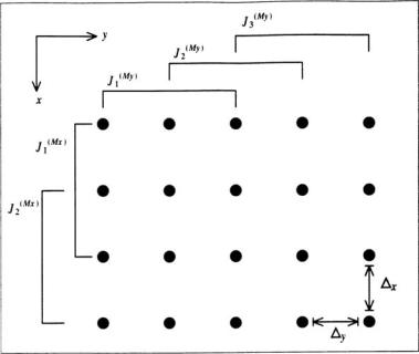
In this section, the method of spatial smoothing is extended to two-dimensional arrays, which are used to find joint azimuthal and elevational angles of a signal source. Two-dimensional spatial smoothing can thus be used as a preprocessing scheme to decorrelate coherent signals and extend the number of available snapshots. The key is to consider the rectangular array as linear arrays in the x and y directions. Then, the smoothing operation can still be applied in the same line as in the one-dimensional case [3, 7, 8].
Consider a URA of size M = 4 × 5 elements as shown in Figure 4.3. The ULA in the y direction contains My = 5 elements. Now, divide
each of these linear arrays into Ly = 3 subarrays. Then each subarray will
have Msub y = M y − Ly + 1 = 3 elements in the y direction, as shown in Figure 4.3.
Preprocessing Schemes and Model Order Estimation |
73 |
|
|
Figure 4.3 An example of two different subarrays for two-dimensional spatial smoothing.
Similarly, ULAs in the x direction contain Mx = 4 elements. By
dividing each of these linear arrays into Lx = 2 subarrays, each subarray |
|||
contains Msub y = M y |
− Ly + 1 = 3 elements in the x direction. |
||
|
As a result, the whole URA of size M = Mx × My elements is divided |
||
into |
L = |
Lx × Ly |
small rectangular subarrays, each containing |
Msub |
= Msub x |
× Msub y |
elements. In this example, we divide an M = 20 ele- |
ment URA into L = 2 × 3 = 6 rectangular subarrays, each having Msub = 3 × 3 = 9 elements.
Once the linear subarrays in the x and y directions are chosen, the selection matrices corresponding to each of these subarrays can be formed. As described before, the one-dimensional selection matrix corresponding to the l xth subarray of ULA in the x direction is defined as
(M x ) |
= [0 I M sub x 0], 1≤ l x ≤ L x |
(4.15) |
Jl x |