Добавил:

Upload Опубликованный материал нарушает ваши авторские права? Сообщите нам.

Вуз:

Санкт-Петербургский государственный университет информационных технологий, механики и оптики

Предмет:

[НЕСОРТИРОВАННОЕ]

Файл:

Rasseyanie_Tuchin.pdf

Скачиваний:

Добавлен:

21.03.2016

Размер:

38.9 Mб

Скачать

☆

<<< < Предыдущая 1 2 3 4 56 / 146 7 8 9 10 11 12 13 14 > Следующая >>>

Methods and Algorithms for the Measurement of the Optical Parameters of Tissues

Methods and algorithms for solving the inverse problem of ﬁnding tissue and blood optical parameters such as absorption and scattering coefﬁcients, anisotropy factor, and refractive index are presented. Advantages and drawbacks of these methods are analyzed. Widespread measuring techniques such as integrating sphere, spatially, time-, and angular-resolved, and OCT, as well as inverse methods, such as Kubelka-Munk, multiﬂux, adding-doubling and inverse Monte Carlo, are overviewed. Exhaustive data on optical properties of human tissue and blood measured in vitro, ex vivo, and in vivo are presented.

2.1 Basic principles

Methods for determining the optical parameters of tissues can be divided into two

large groups, direct and indirect methods.1–4,9–16,29,32,33,37,38,40,46,48,49,56,72,87–90, 98,129,130,164,179,182,213,221,222,226–228,231–233,236–238,255,263,369,572,649–726 Direct

methods include those based on some fundamental concepts and rules such as the Bouguer-Beer-Lambert law [see Eq. (1.1)], the single-scattering phase function [see Eqs. (1.13) and (1.15)] for thin samples, or the effective light penetration depth for slabs. The parameters measured are the collimated light transmission Tc and the scattering indicatrix I (θ) (angular dependence of the scattered light intensity, W/cm2 sr) for thin samples or the ﬂuence rate inside a slab. The normalized scattering indicatrix is equal to the scattering phase function I (θ)/I (0) ≡ p(θ), 1/sr. These methods are advantageous in that they use very simple analytic expressions for data processing. Their disadvantages are related to the necessity to strictly fulﬁll experimental conditions dictated by the selected model (single scattering in thin samples, exclusion of the effects of light polarization and refraction at cuvette edges, etc.); in the case of slabs with multiple scattering, the recording detector (usually a ﬁber light guide with an isotropically scattering ball at the tip end) must be placed far from both the light source and the medium boundaries.

Indirect methods obtain the solution of the inverse scattering problem using a theoretical model of light propagation in a medium. They are in turn divided into iterative and noniterative models. The former use equations in which the optical properties are deﬁned through parameters directly related to

the quantities being evaluated. The latter are based on the two-ﬂux KubelkaMunk model and multiﬂux models.40,46,56,93,183,192,213,255,661,674 In indirect iter-

ative methods, the optical properties are implicitly deﬁned through measured pa-

143

144 Methods and Algorithms for the Measurement of the Optical Parameters of Tissues

rameters. Quantities determining the optical properties of a scattering medium are enumerated until the estimated and measured values for reﬂectance and transmittance coincide with the desired accuracy. These methods are cumbersome, but the optical models currently in use may be even more complicated

than those underlying noniterative methods [examples include the diffusion

theory,40,183,198–203 inverse adding-doubling (IAD),266,267,646,652,667,675–677 and inverse MC (IMC)213,226,236–238,242,244,255,263,264,369,650,655,656,662,665,678,719,720

methods].

The optical parameters of tissue samples (μa, μs, and g) are measured by different methods. In vitro evaluation is most often achieved by the double integrating sphere method combined with collimated transmittance measurements (see Fig. 2.1 and Table 2.1). This approach implies either sequential or simultaneous determination of three parameters: collimated transmittance Tc = I (d)/I (0) [see Eq. (1.1)], total transmittance Tt = Tc + Td (Td being diffuse transmittance), and diffuse reﬂectance Rd. The optical parameters of the tissue are deduced from these measurements using different theoretical expressions or numerical methods (two-ﬂux and multiﬂux models, the IMC or IAD methods) relating μa, μs, and g to the parameters being investigated.

Figure 2.1 Measurement of (a) collimated and (b) total transmittance, and diffuse reﬂectance using an integrating sphere. The integrating surface of the sphere is coated with BaSO4 or MgO, which have nearly 100% diffuse remittance over the entire optical

spectrum.6,57

Any three measurements from the following ﬁve are sufﬁcient for the evaluation of all three optical parameters:40

• Total (or diffuse) transmittance for collimated or diffuse radiation.

Table 2.1 Optical properties of human tissues measured in vitro, ex vivo, and in vivo (rms. values are given in parentheses).

Tissue	λ, nm	μa, cm−1	μs, cm−1	μs, cm−1	g	Remarks
In vitro measurements
Aorta:
Normal	308	33	–	77	–	Post mortem (6 hr), excised, in
Normal coagulated	308	44	–	270	–	4◦C saline, slab, water bath
Fibrous plaque	308	24	–	81	–	(85◦C), integrating sphere (IS)
Fibrous plaque coagulated	308	34	–	272	–	technique, inverse adding
						doubling (IAD) method, data
						from Ref. 40
Normal	1064	0.53 (0.09)	239 (45)	23.9	0.9	Post mortem, slab, 70◦C water
Coagulated	1064	0.46 (0.18)	293 (73)	29.3	0.9	bath, 10 min, IS, inverse Monte
						Carlo (IMC) method,
						goniophotometric
						measurements (GPM), data
						from Ref. 40
Fibro-fatty	355	17.7	–	64.9	–	Post mortem, resected, slab
	532	3.6	–	24.8	–	(24 hr), photoacoustic (PA),
	1064	0.09	–	7.7	–	data from Ref. 40
Normal	633*	0.52	316	41	0.87	Post mortem, slab, IS, GPM,
	1064**	0.5	239	23.9	0.9	diffusion theory (DT), *IMC,
	1064*	0.7	–	22.4	–	data from Ref. 40
	1320**	2.2	233	23.3	0.9
	1320*	4.3	–	17.8	–
Normal	470	5.3 (0.9)	–	42.6 (6.0)	–	Thin sections (250 μm, intima
	476	5.1 (0.9)	–	41.9 (5.9)	–	and media), kept in saline.569
	488	4.5 (0.9)	–	39.9 (5.6)	–	IS, DT.
	514.5	3.7 (0.9)	–	36.9 (5.4)	–	Corrected data (see Ref. 3,
	580	2.8 (0.9)	–	31.1 (4.9)	–	p. 379)
	600	2.6 (0.9)	–	29.6 (4.7)	–

Diagnosis Medical for Instruments and Methods Scattering Light Optics: Tissue

145

			Table 2.1 (Continued).
Tissue	λ, nm	μa, cm−1	μs, cm−1	μs, cm−1	g	Remarks
	633	2.6 (0.9)	–	27.4 (4.4)	–
	1064	2.7 (0.5)	–	15.5 (2.8)	–
Adventitia	476	18.1	267	69.4	0.74	Frozen sections, IS, DT,
	580	11.3	217	49.9	0.77	Ref. 218
	600	6.1	211	46.4	0.78
	633	5.8	195	37.1	0.81
	1064	2.0	484	–	0.97	Double IS (DIS), DT, data
						from Ref. 691
Intima	476	14.8	237	45.0	0.81	Frozen sections, IS, DT,
	580	8.9	183	34.8	0.81	Ref. 218
	600	4.0	178	33.8	0.81
	633	3.6	171	25.7	0.85
	1064	2.3	165	–	0.97	DIS, DT, data from Ref. 691
Media	476	7.3	410	45.1	0.89	Frozen sections, IS, DT,
	580	4.8	331	33.1	0.90	Ref. 218
	600	2.5	323	35.5	0.89
	633	2.3	310	31.0	0.90
	1064	1.0	634	–	0.96	DIS, DT, data from Ref. 691
Bladder:
Integral	633	1.40	88.0	3.52	0.96	Excised, kept in saline, Ref. 40
Integral	633	1.40	29.3	2.64	0.91	DIS, DT, data from Refs. 2
Mucous	1064	0.7	7.5	–	0.85	and 691
Wall	1064	0.9	54.3	–	0.85
Integral	1064	0.4	116	–	0.90
Blood:
HbO2 (Hct = 0.41)	665	1.30	1246	6.11	0.995	Whole blood; absorbance,
HbO2 (Hct = 0.41)	685	2.65	1413	14.13	0.990	radial reﬂectance, and/or GPM;
HbO2 (Hct = 0.41)	960	2.84	505	3.84	0.992	Mie theory, transport theory, or

146

Tissues of Parameters Optical the of Measurement the for Algorithms and Methods

					Table 2.1 (Continued).
Tissue	λ, nm	μa, cm−1		μs, cm−1		μs, cm−1	g	Remarks
HbO2 (Hct = 0.4)	810	4.5		–		6.6	–	IMC; data from Refs. 691
HbO2 (Hct = 0.4)	1064	3.0		–		3.4	–	and 40
Hb (Hct = 0.41)	960	16.8		668		5.08	0.992
Hb (Hct = 0.4)	810	4.5		–		3.9	–
Hb (Hct = 0.4)	1064	0.3		–		6.6	–
Hct = 0.47	450	381		2940		8.3	0.9972	Whole blood; IAD and Beer’s
(partially oxygenated)	488	133		3190		4.0	0.9987	law; data by Jacques (1993)
	514	116		3320		4.1	0.9988	from Ref. 40
	577	301		3140		7.3	0.9977
	630	14.3		3660		8.9	0.9976
(Hct = 0.45–0.46,	760	15.5		2820		7.9	0.9972
(Hct = 0.45–0.46,	633	15.5		644.7		–	0.982	DIS, Henyey-Greenstein phase
oxygenation > 98%)	710	4 (0.8)		737	(75)	–	0.986 (0.006)	function (HGPF), IMC,665,666
	765	5.3	(0.6)	725	(75)	–	0.991 (0.002)	data from graphs of
	810	6.5	(0.5)	690	(80)	–	0.989 (0.002)	Refs. 164, 724; whole blood
	865	7.2	(0.3)	649	(25)	–	0.990 (0.001)
	910	8.9	(0.4)	649	(25)	–	0.992 (0.002)
	965	9.3	(0.6)	650	(25)	–	0.991 (0.001)
	1010	8.3	(0.4)	645	(25)	–	0.992 (0.001)
	1065	5.6	(0.3)	645	(25)	–	0.992 (0.001)
	1110	4.2	(0.3)	630	(20)	–	0.993 (0.001)
	1165	4.1	(0.7)	655	(15)	–	0.993 (0.001)
(Hct = 0.421,	1210	5.5	(0.5)	654	(20)	–	0.995 (0.001)
(Hct = 0.421,	260	375.5	(9.0)	631.5 (57.6)		136.4 (28.0)	0.784 (0.030)	IS, fresh erythrocytes from a
oxygenation > 99%)	350	368.1		559.5		82.5	0.852	healthy blood donor diluted in
	375	338.6	(4.2)	542.8 (66.5)		69.5 (12.7)	0.872 (0.007)	PBS, pH 7.4, hemoglobin
	415	782.5	(62.9)	390.3 (61.2)		129.5 (17.0)	0.668 (0.008)	concentration 129 g/l, the
	450	263.0		682.6		52.5	0.923	temperature was kept constant

Diagnosis Medical for Instruments and Methods Scattering Light Optics: Tissue

147

				Table 2.1 (Continued).
Tissue	λ, nm	μa, cm−1		μs, cm−1	μs, cm−1	g	Remarks
	490	106.8		793.8	30.4	0.962	at 20◦C, turbulence-free cuvette
	520	120.4	(6.9)	766.2 (42.4)	24.9 (7.6)	0.967 (0.009)	with a laminar ﬂow and a
	540	232.3		655.6	35.8	0.945	sample thickness of 116 μm,
	555	178.9		709.3	33.0	0.953	constant wall share rate of
	575	231.6		658.0	31.7	0.952	600 s−1; in the wavelength
	585	160.2	(10.3)	751.7 (46.1)	33.5 (9.7)	0.955 (0.007)	region around 415 nm a cuvette
	620	4.14		905.3	23.3	0.974	of 40 μm in thickness was used;
	630	2.51 (0.09)		894.6 (28.6)	22.3 (3.3)	0.975 (0.004)	Reynolds-McCormick phase
	670	1.22		892.3	21.5	0.976	function (α = 1.7), IMC, data
	700	1.25		879.3	21.1	0.976	were presented by the authors of
	750	1.99		840.8	20.6	0.975	were presented by the authors of
	750	1.99		840.8	20.6	0.975	Ref. 1271.
	780	2.85		821.5	20.5	0.975	Ref. 1271.
	780	2.85		821.5	20.5	0.975
	800	3.27 (0.12)		809.9 (66.4)	20.2 (5.4)	0.975 (0.003)
	830	4.90		798.7	20.1	0.975
	850	4.65		799.5	20.1	0.975
	870	5.10		784.4	20.1	0.974
	900	5.43		751.4	19.9	0.973
	950	6.15 (0.35)		712.0 (69.8)	20.8 (2.7)	0.971 (0.002)
	980	6.79		685.9	20.8	0.970
	1000	6.51		680.8	20.5	0.970
	1050	4.91 (0.12)		661.3 (12.8)	19.91 (0.67)	0.9699 (0.0006)
	1100	3.74		639.5	18.85	0.970
Brain:		10*		84*		0.9*
Astrocytoma (grade III	400	10*		84*	–	0.9*	Microspectrophotometry, IMC,
WHO, n = 7, different	633	6.3	(1.6)	67 (8)	–	0.883 (0.011)	slab 600 μm,263
spots on the sample)	700	4*		50*	–	0.88*	* data from graphs
	800	3*		50*	–	0.88*
Glioma	415	16.6		–	6		Ref. 39, data from graphs

148

Tissues of Parameters Optical the of Measurement the for Algorithms and Methods

			Table 2.1 (Continued).
Tissue	λ, nm	μa, cm−1	μs, cm−1	μs, cm−1		g	Remarks
(male, 65 yr,	488	12.5	–	3		–
4 hr post mortem)	630	3.0	–	3		–
	800–1100	≈1.0	–	>1–2		–
Gray matter	514	19.5	–	85		–
(male, 71 yr,	585	14.5	–	63		–
24 hr post mortem)	630	4.3	–	52		–
	800–1100	≈1.0	–	45–20		–
Melanoma	585	2	–	158		–
(male 71 yr,	630	20.0	–	75		–
24 hr post mortem)	800	8.0	–	40		–
	900	4.0	–	30		–
	1100	2.0	–	25		–
White matter	415	2.1	–	24		–
(female, 32 yr,	488	1.0	–	60		–
24 hr post mortem)	630	0.2	–	32		–
	800–1100	0.2–0.3	–	40–20		–
White matter	488	2.7	–	25		–
(female, 63 yr,	630	0.9	–	22		–
30 hr post mortem)	800–1100	1.0–1.5	–	20–10		–
Gray matter	633	2.7 (2)	354 (37)	20.6 (2)		0.94 (0.004)	Freshly resected, slabs; data
	1064	5.0 (5)	134 (14)	11.8 (9)		0.90 (0.007)	from Ref. 40
White matter	633	2.2 (2)	532 (41)	91	(5)	0.82 (0.01)
	1064	3.2 (4)	469 (34)	60.3 (2.5)		0.87 (0.007)
Gray matter	800	0.25	–	25		–	Ref. 233
White matter	800	0.05	–	60		–
Gray matter (n = 7)	360	3.33 (2.19)	141.3 (42.6)	–		0.818 (0.093)	DIS, IMC665,666
	640	0.17 (0.26)	90.1 (32.5)	–		0.89 (0.04)
	1060	0.56 (0.7)	56.8 (18.0)	–		0.90 (0.05)

Diagnosis Medical for Instruments and Methods Scattering Light Optics: Tissue

149

				Table 2.1 (Continued).
Tissue	λ, nm	μa, cm−1		μs, cm−1		μs, cm−1	g	Remarks
Gray matter coagulated (n = 7)	360	9.39 (1.70)		426	(122)	–	0.868 (0.031)	DIS, IMC; 2 hr, 80◦C665,666
	740	0.45 (0.27)		–		–	–
	1100	1.0	(0.45)	179.8 (32.6)		–	0.954 (0.001)
Gray matter	456	9		686		34.3	0.95	IS, δ-Eddington
	514	11.7		578		17.34	0.97	approximation;698
	630	1.4		473		33.11	0.93	data from Ref. 264
	675	0.6		364		32.76	0.91
	1064	1.9		267		10.7	0.96
White matter	456	8.1		923		73.84	0.92
	514	5.0		1045		73.15	0.93
	630	1.5		386		54.04	0.86
	675	0.7		436		56.68	0.87
White matter (n = 7)	1064	1.6		513		25.65	0.95	DIS, IMC665,666
White matter (n = 7)	360	2.53 (0.55)		402.0 (91.8)		–	0.702 (0.093)	DIS, IMC665,666
	640	0.8	(0.2)	408.2 (88.5)		–	0.84 (0.05)
	860	0.97 (0.4)		353.1 (68.1)		–	0.871 (0.028)
White matter coagulated (n = 7)	1060	1.08 (0.51)		299.5 (70.1)			0.889 (0.010)	DIS, IMC; 2 hr, 80◦C665,666
White matter coagulated (n = 7)	360	8.3	(3.65)	604.2 (131.5) –			0.800 (0.089)	DIS, IMC; 2 hr, 80◦C665,666
	860	1.7	(1.3)	417.0 (272.5) –			0.922 (0.025)
	1060	2.15 (1.34)		363.3 (226.8) –			0.930 (0.015)
White matter	800	0.8	(0.16)	140	(14)	–	0.95 (0.02)	DIS, IMC; samples 0.5–3 hr
	1064	0.4	(0.08)	110	(11)	–	0.95 (0.02)	post mortem, fast frozen and
White matter coagulated	800	0.9	(0.18)	170	(17)	10.2	0.94 (0.02)	homogenized; coagulation in
Gray matter (n = 7)	1064	0.5	(0.1)	130	(13)	9.1	0.93 (0.02)	a bath at 75◦C 662
Gray matter (n = 7)	450	0.7		117		14.04	0.88	IS, IMC, quasi-Newton inverse
	510	0.4		106		12.72	0.88	algorithm,
	630	0.2		90		9.9	0.89	HGPF;

150

Tissues of Parameters Optical the of Measurement the for Algorithms and Methods

				Table 2.1 (Continued).
Tissue	λ, nm	μa, cm−1		μs, cm−1	μs, cm−1	g	Remarks
	670	0.2		84	8.4	0.90	hemoglobin free cryosections
White matter (n = 7)	1064	0.5		57	5.7	0.90	(<48 hr post mortem): gray
White matter (n = 7)	450	1.4		420	92.4	0.78	matter—100–200 μm; white
	510	1.0		426	80.94	0.81	matter—80–150 μm;
	630	0.8		409	65.44	0.84	coagulation: saline bath 80◦C,
	670	0.7		401	60.15	0.85	2 hr;264 data from tables of
	850	1.0		342	41	0.88	Ref. 264
White matter coagulated (n = 7)	1064	1.0		296	32.56	0.89
White matter coagulated (n = 7)	850	0.9		300	36.0	0.88
	1064	0.1		270	29.7	0.89
Astrocytoma (grade II WHO,	400	18.8	(11.3)	198.4 (55.6)	–	0.93 (0.03)	IS, IMC, quasi-Newton inverse
n = 4)	490	2.5	(0.9)	158.5 (53.7)	–	0.96 (0.02)	algorithm,
	600	1.2	(0.7)	132.4 (49.0)	–	0.96 (0.02)	HGPF;
	700	0.5	(0.3)	113.2 (41.8)	–	0.96 (0.02)	hemoglobin free cryosections of
	800	0.7	(0.2)	96.7 (41.8)	–	0.96 (0.01)	normal tissues (<48 hr post
	900	0.3	(0.2)	86.4 (34.6)	–	0.96 (0.01)	mortem): cerebellum, gray
	1000	0.5	(0.3)	79.0 (34.2)	–	0.96 (0.01)	matter, pons, and
Cerebellum (n = 7)	1100	0.6	(0.2)	73.8 (29.6)	–	0.96 (0.01)	thalamus—100–200 μm; white
Cerebellum (n = 7)	400	4.7	(0.8)	276.7 (19.1)	–	0.80 (0.03)	matter—80–150 μm; and
	500	1.4	(0.2)	277.5 (32.6)	–	0.85 (0.02)	tumors excised from patients of
	600	0.8	(0.2)	272.1 (12.3)	–	0.87 (0.02)	≈300 μm in thickness;
	700	0.6	(0.1)	266.8 (12.1)	–	0.89 (0.01)	coagulation: saline bath 80◦C,
	800	0.6	(0.1)	250.3 (17.2)	–	0.90 (0.01)	2 hr;264 data from graphs of
	900	0.7	(0.1)	229.6 (15.8)	–	0.90 (0.01)	Ref. 264, taken from Ref. 696
	1000	0.8	(0.1)	215.4 (14.7)	–	0.90 (0.01)	with corrections
Cerebellum coagulated (n = 7)	1100	0.7	(0.1)	202.1 (13.9)	–	0.90 (0.01)
Cerebellum coagulated (n = 7)	400	19.3	(7.7)	560.0 (25.5)	–	0.61 (0.01)
	500	5.1	(1.7)	512.2 (47.8)	–	0.77 (0.02)

Diagnosis Medical for Instruments and Methods Scattering Light Optics: Tissue

151

Table 2.1 (Continued).	152

Tissue	λ, nm	μa, cm−1	μs, cm−1		μs, cm−1	g		Remarks
	600	2.9 (1.4)	458.2	(65.6)	–	0.78 (0.01)
	700	1.7 (0.4)	489.9	(70.1)	–	0.85 (0.01)
	800	1.1 (0.2)	458.2	(54.0)	–	0.87 (0.02)			Methods
	900	1.1 (0.3)	458.2	(65.6)	–	0.89	(0.02)

	1000	1.0 (0.4)	419.1	(49.4)	–	0.90 (0.03)
Gray matter (n = 7)	1100	1.1 (0.5)	428.5	(40.0)	–	0.91 (0.03)			and
	400	2.6 (0.6)	128.5	(18.4)	–	0.87	(0.02)
									Algorithms
	500	0.5 (0.2)	109.9	(13.0)	–	0.88	(0.01)

	600	0.3 (0.1)	94.1	(13.5)	–	0.89 (0.02)
	700	0.2 (0.1)	84.1	(12.0)	–	0.90 (0.02)
	800	0.2 (0.1)	77.0	(11.0)	–	0.90 (0.02)			for
	900	0.3 (0.2)	67.3	(9.6)	–	0.90	(0.02)
									the
	1000	0.6 (0.3)	61.6	(5.7)	–	0.90	(0.02)
									Measurement
Gray matter coagulated (n = 7)	1100	0.5 (0.3)	55.1	(6.5)	–	0.90	(0.02)

	400	7.5 (0.4)	258.6	(18.8)	–	0.78 (0.04)
	500	1.8 (0.2)	326.5	(7.7)	–	0.85 (0.03)
	600	0.7 (0.1)	319.0	(15.2)	–	0.87 (0.03)			of
	700	0.7 (0.1)	319.0	(7.5)	–	0.88	(0.03)
									the
	800	0.8 (0.1)	252.7	(18.3)	–	0.87	(0.02)
									Optical
	1000	1.4 (0.2)	191.0	(18.7)	–	0.88	(0.03)
	900	0.9 (0.1)	214.6	(10.3)	–	0.87	(0.02)
Meningioma (n = 6)	1100	1.5 (0.2)	186.6	(13.5)	–	0.88 (0.03)			Parameters
	410	4.1 (0.5)	197.4	(19.8)	–	0.88	(0.02)

	490	1.3 (0.2)	188.2	(18.8)	–	0.93 (0.01)
	590	0.7 (0.2)	171.1	(12.7)	–	0.95 (0.01)			of
	690	0.3 (0.1)	155.5	(15.6)	–	0.95	(0.01)
									Tissues
	790	0.2 (0.1)	141.3	(14.2)	–	0.96	(0.01)

			Table 2.1 (Continued).
Tissue	λ, nm	μa, cm−1	μs, cm−1		μs, cm−1	g	Remarks
	910	0.2 (0.1)	116.8	(8.6)	–	0.95 (0.01)
	990	0.4 (0.2)	163.5	(15.3)	–	0.96 (0.01)
Pons (n = 7)	1100	0.6 (0.2)	133.7	(19.2)	–	0.97 (0.01)
Pons (n = 7)	400	3.1 (0.7)	163.5	(15.3)	–	0.89 (0.02)
	500	0.9 (0.3)	133.7	(19.2)	–	0.91 (0.01)
	600	0.6 (0.2)	109.4	(18.5)	–	0.91 (0.01)
	700	0.5 (0.2)	93.5	(20.9)	–	0.91 (0.01)
	800	0.6 (0.3)	83.6	(21.0)	–	0.91 (0.01)
	900	0.7 (0.3)	74.8	(18.7)	–	0.92 (0.01)
	1000	1.0 (0.4)	69.9	(17.5)	–	0.91 (0.01)
Pons coagulated (n = 7)	1100	0.9 (0.4)	64.0	(17.8)	–	0.92 (0.01)
Pons coagulated (n = 7)	410	17.2 (1.6)	685.7	(63.7)	–	0.85 (0.02)
	510	8.5 (0.8)	627.5	(73.6)	–	0.89 (0.01)
	610	7.7 (0.5)	510.5	(70.5)	–	0.89 (0.01)
	710	6.9 (0.6)	402.5	(67.7)	–	0.89 (0.01)
	810	6.5 (0.6)	329.7	(55.4)	–	0.89 (0.01)
	910	5.9 (1.0)	276.0	(46.4)	–	0.88 (0.01)
	1010	5.7 (1.0)	241.6(34.4)		–	0.88 (0.01)
Thalamus (n = 7)	1100	6.5 (0.9)	221.1	(31.5)	–	0.88 (0.01)
Thalamus (n = 7)	410	3.2 (1.0)	146.7	(49.4)	–	0.86 (0.03)
	510	0.9 (0.3)	188.7	(31.9)	–	0.87 (0.03)
	610	0.6 (0.2)	176.3	(34.5)	–	0.88 (0.02)
	710	0.5 (0.3)	169.0	(28.7)	–	0.89 (0.03)
	810	0.7 (0.3)	158.5	(35.3)	–	0.89 (0.02)
	910	0.7 (0.3)	155.4	(22.3)	–	0.90 (0.02)
	1010	0.8 (0.3)	139.3	(34.9)	–	0.90 (0.02)
	1100	0.8 (0.3)	146.0	(36.6)	–	0.91 (0.02)

Diagnosis Medical for Instruments and Methods Scattering Light Optics: Tissue

153

			Table 2.1 (Continued).
Tissue	λ, nm	μa, cm−1	μs, cm−1	μs, cm−1	g	Remarks
Thalamus coagulated (n = 7)	400	15.0 (3.3)	391.1 (56.1)	–	0.83 (0.04)
	500	4.2 (0.9)	399.9 (67.7)	–	0.90 (0.01)
	600	1.6 (0.6)	365.7 (43.2)	–	0.92 (0.01)
	700	1.4 (0.3)	327.0 (30.6)	–	0.92 (0.01)
	800	1.1 (0.3)	286.0 (33.8)	–	0.93 (0.01)
	900	1.1 (0.3)	267.4 (31.6)	–	0.93 (0.01)
	1000	1.4 (0.4)	233.8 (39.7)	–	0.93 (0.01)
White matter (n = 7)	1100	1.5 (0.4)	223.6 (32.1)	–	0.94 (0.01)
White matter (n = 7)	400	3.1 (0.2)	413.5 (21.4)	–	0.75 (0.03)
	500	0.9 (0.1)	413.5 (43.9)	–	0.80 (0.02)
	600	0.8 (0.1)	413.5 (21.4)	–	0.83 (0.02)
	700	0.8 (0.1)	393.1 (30.9)	–	0.85 (0.02)
	800	0.9 (0.1)	364.5 (28.6)	–	0.87 (0.01)
	900	1.0 (0.1)	329.5 (35.0)	–	0.88 (0.01)
	1000	1.2 (0.2)	305.4 (15.9)	–	0.88 (0.01)
White matter coagulated (n = 7)	1100	1.0 (0.2)	283.2 (22.2)	–	0.88 (0.01)
White matter coagulated (n = 7)	410	8.7 (1.7)	568.7 (111.9)	–	0.83 (0.03)
	510	2.9 (0.6)	513.2 (116.9)	–	0.87 (0.02)
	610	1.7 (0.4)	500.2 (129.9)	–	0.90 (0.02)
	710	1.4 (0.5)	475.2 (108.3)	–	0.91 (0.01)
	810	1.5 (0.5)	440.0 (114.3)	–	0.92 (0.01)
	910	1.7 (0.6)	407.4 (92.8)	–	0.93 (0.01)
	1010	1.9 (0.6)	367.7 (95.5)	–	0.93 (0.01)
Gray matter (n = 25)	1100	2.4 (0.5)	358.4 (81.6)	–	0.93 (0.01)
Gray matter (n = 25)	400	9.778	–	25.878	–	IS, IAD, ﬁxed the anisotropy factor
	418	14.873	–	26.593	–	g = 0.85 and the refractive index
	428	16.722	–	26.709	–	n = 1.40 were assumed for every

154

Tissues of Parameters Optical the of Measurement the for Algorithms and Methods

			Table 2.1 (Continued).
Tissue	λ, nm	μa, cm−1	μs, cm−1	μs, cm−1	g	Remarks
	450	5.161	–	19.389	–	wavelength and for every sample; brain
	488	2.272	–	15.957	–	tissue samples were acquired during open
	500	2.206	–	15.283	–	craniotomy for tumor resection or temporal
	550	2.955	–	13.315	–	lobectomy, hemoglobin free cryosections
	600	1.460	–	11.367	–	with thickness from 0.22 to 1.25 mm were
	632	0.925	–	10.370	–	studied, measurements were done at 25◦C,
	670	0.809	–	9.480	–	pH 7.4; data were presented by the authors
	700	0.733	–	8.907	–	of Ref. 1272
	750	0.599	–	8.481	–
	800	0.507	–	7.886	–
	830	0.485	–	7.707	–
	850	0.472	–	7.555	–
	870	0.479	–	7.351	–
	900	0.503	–	7.055	–
	950	0.521	–	6.868	–
	1000	0.585	–	6.059	–
	1064	0.502	–	5.333	–
	1100	0.502	–	5.197	–
	1150	0.815	–	5.070	–
	1200	1.010	–	4.882	–
	1250	0.865	–	4.669	–
White matter (n = 19)	1300	0.894	–	4.560	–
White matter (n = 19)	400	9.134	–	88.611	–
	418	13.603	–	83.304	–
	428	15.417	–	80.905	–
	450	3.958	–	77.053	–
	488	1.869	–	70.112	–
	500	1.834	–	68.318	–

Diagnosis Medical for Instruments and Methods Scattering Light Optics: Tissue

155

			Table 2.1 (Continued).
Tissue	λ, nm	μa, cm−1	μs, cm−1	μs, cm−1	g	Remarks
	550	2.584	–	62.383	–
	600	1.175	–	56.759	–
	632	0.801	–	53.179	–
	670	0.711	–	50.067	–
	700	0.674	–	47.626	–
	750	0.649	–	45.061	–
	800	0.622	–	41.878	–
	830	0.626	–	40.634	–
	850	0.643	–	39.658	–
	870	0.666	–	38.785	–
	900	0.684	–	37.607	–
	950	0.785	–	35.851	–
	1000	0.883	–	32.603	–
	1064	0.752	–	30.161	–
	1100	0.762	–	29.219	–
	1150	1.135	–	27.951	–
	1200	1.420	–	26.646	–
	1250	1.268	–	25.310	–
Glioma (n = 39)	1300	1.274	–	24.250	–
Glioma (n = 39)	400	12.393	–	39.009	–
	418	17.496	–	37.867	–
	428	16.124	–	37.076	–
	450	4.891	–	32.340	–
	488	2.592	–	28.933	–
	500	2.352	–	28.057	–
	550	2.768	–	25.300	–
	600	1.149	–	22.514	–
	632	0.846	–	21.068	–

156

Tissues of Parameters Optical the of Measurement the for Algorithms and Methods

		Table 2.1 (Continued).
Tissue	λ, nm	μa, cm−1	μs, cm−1	μs, cm−1	g	Remarks
	670	0.741	–	19.608	–
	700	0.709	–	18.543	–
	750	0.679	–	17.343	–
	800	0.656	–	15.969	–
	830	0.662	–	15.481	–
	850	0.670	–	15.133	–
	870	0.685	–	14.749	–
	900	0.707	–	14.138	–
	950	0.768	–	13.646	–
	1000	0.938	–	11.588	–
	1064	0.822	–	10.344	–
	1100	0.831	–	10.005	–
	1150	1.231	–	9.654	–
	1200	1.518	–	9.282	–
	1250	1.379	–	8.813	–
	1300	1.412	–	8.523	–
Breast (female):						Excised, kept in saline, 37◦C,
Fatty normal	749	0.18 (0.16)	8.48 (3.43)	–	–	Excised, kept in saline, 37◦C,
(n = 23)	789	0.08 (0.10)	7.67 (2.57)	–	–	Ref. 232
Fibrous normal (n = 35)	836	0.11 (0.10)	7.27 (2.40)	–	–
Fibrous normal (n = 35)	749	0.13 (0.19)	9.75 (2.27)	–	–
	789	0.06 (0.12)	8.94 (2.45)	–	–
Inﬁltrating carcinoma (n = 48)	836	0.05 (0.08)	8.10 (2.21)	–	–
Inﬁltrating carcinoma (n = 48)	749	0.15 (0.14)	10.91 (5.59)	–	–
	789	0.04 (0.08)	10.12 (5.05)	–	–
Mucinous carcinoma (n = 3)	836	0.10 (0.19)	9.10 (4.54)	–	–
Mucinous carcinoma (n = 3)	749	0.26 (0.20)	–	6.15 (2.44)	–
	789	0.016 (0.072)	–	5.09 (2.42)	–

Diagnosis Medical for Instruments and Methods Scattering Light Optics: Tissue

157

			Table 2.1 (Continued).
Tissue	λ, nm	μa, cm−1	μs, cm−1	μs, cm−1	g	Remarks
	836	0.023 (0.108)	–	4.78 (3.67)	–
Ductal carcinoma	749	0.076 (0.068)	–	13.10 (2.85)	–
in situ (n = 5)	789	0.023 (0.034)	–	12.21 (2.45)	–
Glandular tissue (n = 3)	836	0.039 (0.068)	–	10.46 (2.65)	–
Glandular tissue (n = 3)	540	3.58 (1.56)	–	24.4 (5.8)	–	Homogenized tissue, Ref. 660
	700	0.47 (0.11)	–	14.2 (3.0)	–
Fatty tissue (n = 7)	900	0.62 (0.05)	–	9.9 (2.0)	–
Fatty tissue (n = 7)	540	2.27 (0.57)	–	10.3 (1.9)	–
	700	0.70 (0.08)	–	8.6 (1.3)	–
Fibrocystic (n = 8)	900	0.75 (0.08)	–	7.9 (1.1)	–
Fibrocystic (n = 8)	540	1.64 (0.66)	–	21.7 (3.3)	–
	700	0.22 (0.09)	–	13.4 (1.9)	–
Fibroadenoma (n = 6)	900	0.27 (0.11)	–	9.5 (1.7)	–
Fibroadenoma (n = 6)	540	4.38 (3.14)	–	11.1 (3.0)	–
	700	0.52 (0.47)	–	7.2 (1.7)	–
Carcinoma (n = 9)	900	0.72 (0.53)	–	5.3 (1.4)	–
Carcinoma (n = 9)	540	3.07 (0.99)	–	19.0 (5.1)	–
	700	0.45 (0.12)	–	11.8 (3.1)	–
	900	0.50 (0.15)	–	8.9 (2.6)	–
Carcinoma	580	4.5 (0.8)	–	–	–	Tissue slices of thickness
	850	0.4 (0.5)	–	–	–	5–5.3 mm, Ref. 223
	1300	0.5 (0.8)	–	–	–
Adjacent healthy tissue	580	2.6 (1.1)	–	–	–
	850	0.3 (0.2)	–	–	–
	1300	0.8 (0.6)	–	–	–
Fatty tissue	700	–	–	13 (5)	0.95 (0.02)
Fibroglandular tissue	700	–	–	12 (5)	0.92 (0.03)
Carcinoma (central part)	700	–	–	18 (5)	0.88 (0.03)

158

Tissues of Parameters Optical the of Measurement the for Algorithms and Methods

			Table 2.1 (Continued).
Tissue	λ, nm	μa, cm−1	μs, cm−1	μs, cm−1	g	Remarks
Fatty tissue	625	0.06 (0.02)	–	14.3 (2.1)	–	Ref. 31
Benign tumor	625	0.33 (0.06)	–	3.8 (0.3)	–
Invasive ductal	450	2.55 (0.30)	–	31.5 (2.5)	–	Spatially resolved reﬂectance
carcinoma (n = 10, 9 in	460	2.62 (0.34)	–	31.0 (2.4)	–	(SRR); diffusion approximation;
the age group 55–65 yr	470	2.44 (0.25)	–	30.7 (2.2)	–	source-detector separation,
and 1–35 yr)	480	2.32 (0.26)	–	30.3 (2.4)	–	rsd > 1.2 mm; ﬁbers with core
	490	2.23 (0.25)	–	29.9 (2.4)	–	diameter 400 μm; tissue slices
	500	2.22 (0.22)	–	29.5 (2.2)	–	of thickness 10 mm699
	510	2.16 (0.24)	–	29.1 (2.3)	–
	520	2.12 (0.22)	–	29.0 (2.3)	–
	530	2.07 (0.22)	–	28.7 (2.0)	–
	540	1.99 (0.21)	–	28.0 (2.1)	–
	550	2.13 (0.23)	–	28.4 (2.0)	–
	560	2.09 (0.21)	–	27.7 (2.0)	–
	570	2.09 (0.25)	–	27.5 (1.9)	–
	580	2.07 (0.21)	–	27.3 (2.0)	–
	590	2.01 (0.22)	–	27.1 (1.7)	–
	600	1.90 (0.19)	–	26.8 (1.8)	–
	610	1.82 (0.18)	–	26.8 (1.6)	–
	620	1.71 (0.18)	–	2.64 (1.8)	–
	630	1.64 (0.17)	–	26.2 (1.5)	–
	640	1.55 (0.17)	–	25.9 (1.4)	–
	650	1.48 (0.15)	–	25.7 (1.3)	–
	633	–	–	–	0.96 (0.01)	GPM, tissue slices of 20 μm;
						HGPF; θ = 10◦–165◦; radius of

Mie scatterer—

aM = 0.64 (0.06) μm699

Diagnosis Medical for Instruments and Methods Scattering Light Optics: Tissue

159

			Table 2.1 (Continued).
Tissue	λ, nm	μa, cm−1	μs, cm−1	μs, cm−1	g	Remarks
	633	–	–	–	0.86 (0.02)	GPM, tissue slices of 20 μm;
						double HGPF
						[g = f (1 − g1) + (1 − f )g2];
						θ = 52◦–165◦;
						aM = 0.28 (0.02) μm699
Adjacent healthy tissue	450	1.45 (0.22)	–	21.7 (2.1)	–	SRR; diffusion approximation;
(n = 10; 9 in the age	460	1.48 (0.21)	–	21.3 (2.2)	–	rsd > 1.2 mm; ﬁbers with core
group 55–65 yr and	470	1.42 (0.21)	–	20.8 (1.9)	–	diameter 400 μm; tissue slices
1–35 yr)	480	1.35 (0.19)	–	20.3 (1.8)	–	of thickness 10 mm699
	490	1.26 (0.21)	–	19.9 (2.0)	–
	500	1.24 (0.21)	–	20.1 (1.8)	–
	510	1.23 (0.19)	–	19.1 (1.9)	–
	520	1.19 (0.18)	–	18.7 (1.8)	–
	530	1.14 (0.17)	–	18.4 (1.8)	–
	540	1.19 (0.22)	–	18.0 (1.8)	–
	550	1.16 (0.26)	–	18.2 (1.6)	–
	560	1.14 (0.17)	–	17.4 (1.5)	–
	570	1.13 (0.16)	–	17.2 (1.5)	–
	580	1.17 (0.17)	–	16.9 (1.3)	–
	590	1.07 (0.17)	–	16.6 (1.4)	–
	600	1.00 (0.12)	–	16.4 (1.5)	–
	610	0.95 (0.12)	–	16.2 (1.5)	–
	620	0.89 (0.11)	–	15.9 (1.3)	–
	630	0.82 (0.07)	–	15.7 (1.3)	–
	640	0.79 (0.08)	–	15.5 (1.2)	–
	650	0.74 (0.08)	–	15.3 (1.2)	–

160

Tissues of Parameters Optical the of Measurement the for Algorithms and Methods

				Table 2.1 (Continued).
Tissue	λ, nm	μa, cm−1		μs, cm−1	μs, cm−1	g	Remarks
	633	–		–	–	0.88 (0.01)	GPM, tissue slices of 20 μm;
							HGPF; θ = 10◦–165◦;
							aM = 0.32 (0.02) μm699
	633	–		–	–	0.76 (0.01)	GPM, tissue slices of 20 μm;
							double HGPF
							[g = f (1 − g1) + (1 − f )g2];
							θ = 52◦–165◦;
Colon:							aM = 0.19 (0.02) μm699
Colon:
Muscle	1064	3.3		238	–	0.93	Data from Ref. 691
Submucous	1064	2.3		117	–	0.91
Mucous	1064	2.7		39	–	0.91
Integral	1064	0.4		261	–	0.94
Esophagus	633	0.4		–	12	–	2.5-mm slab, Ref. 40
Esophagus (mucous)	1064	1.1		83	–	0.86	Data from Ref. 691
Fat:
Abdominal	1064	3.0		37	–	0.91	Data from Ref. 691
Subcutaneous	1064	2.6		29	–	0.91
Gallstones:
Porcinement	351	102	(16)	–	–	–	Dehydrated, embedded in
	488	179	(28)	–	–	–	plastic, and sliced in 1-mm slab,
	580	125	(29)	–	–	–	pulsed photothermal radiometry
	630	85	(11)	–	–	–	technique, data from Ref. 40
	1060	121	(12)	–	–	–
Cholesterol	351	88	(7)	–	–	–
	488	62	(15)	–	–	–
	580	36	(7)	–	–	–

Diagnosis Medical for Instruments and Methods Scattering Light Optics: Tissue

161

			Table 2.1 (Continued).
Tissue	λ, nm	μa, cm−1	μs, cm−1	μs, cm−1	g	Remarks
	630	44 (10)	–	–	–
	1060	60 (9)	–	–	–
Head (adult):
Dura mater (n = 8), post	400	3.08 (0.15)	–	22.35 (0.89)	–	IS, IAD; excised tissue slabs,
mortem, <24 hr	450	1.51 (0.08)	–	22.89 (0.92)	–	stored at −12◦C; measurements
	500	1.09 (0.05)	–	21.60 (0.86)	–	at room temperature; in the
	550	1.10 (0.05)	–	18.48 (0.74)	–	spectral ranges 480–550 and
	600	0.80 (0.04)	–	17.11 (0.68)	–	600–700 nm:
	650	0.70 (0.04)	–	15.51 (0.62)	–	μ = 4.54 × 104λ−1.23,
						s
	700	0.74 (0.04)	–	13.99 (0.56)	–	[λ] = nm; Refs. 703 and 704
Scalp and skull	800	0.4	–	20	–	Ref. 233
Cerebral spinal ﬂuid	800	0.01	–	0.1	–
Scalp (n = 3)	805	0.52 (0.04)	–	14.09 (1.74)	–	Adult scalp post mortem
	900	0.40 (0.02)	–	15.66 (2.06)	–	(<12 hr), excised, slab, IS,
	950	0.39 (0.03)	–	16.44 (2.63)	–	IAD; data averaged for three
	1000	0.33 (0.03)	–	16.83 (2.77)	–	tissue samples with thicknesses
	1100	0.19 (0.04)	–	17.10 (2.69)	–	of 6 ± 0.5 mm, 3.5 ± 0.15 mm
	1200	0.65 (0.04)	–	16.70 (2.89)	–	and 3.5 ± 0.12 mm738,739
	1300	0.50 (0.07)	–	14.70 (2.59)	–
	1400	1.98 (0.31)	–	14.28 (3.69)	–
	1430	2.19 (0.29)	–	13.15 (3.07)	–
	1500	2.04 (0.35)	–	14.40 (3.75)	–
	1600	1.43 (0.22)	–	14.16 (3.41)	–
	1700	1.87 (0.28)	–	14.71 (3.51)	–
	1800	1.73 (0.22)	–	13.36 (2.91)	–
	1900	2.57 (0.28)	–	12.15 (3.05)	–
	1930	2.52 (0.25)	–	11.52 (2.57)	–
	2000	2.09 (0.29)	–	12.00 (2.91)	–

162

Tissues of Parameters Optical the of Measurement the for Algorithms and Methods

			Table 2.1 (Continued).
Tissue	λ, nm	μa, cm−1	μs, cm−1	μs, cm−1	g	Remarks
Scull bone (n = 8)	801	0.11 (0.02)	–	19.48 (1.52)	–	Adult head post mortem (24 hr),
	900	0.15 (0.02)	–	18.03 (1.19)	–	excised, slab from the occipital
	980	0.23 (0.03)	–	17.38 (1.01)	–	part, IS, IAD; data averaged for
	1000	0.22 (0.03)	–	17.10 (0.91)	–	8 tissue samples
	1100	0.16 (0.03)	–	15.92 (0.76)	–	μ = 1.53 × 103λ−0.65,
						s
	1180	0.67 (0.07)	–	16.53 (0.83)	–	[λ] = nm (spectral range from
	1200	0.67 (0.07)	–	16.77 (0.85)	–	1130 to 1910 nm is
	1300	0.54 (0.05)	–	14.78 (0.80)	–	excluded)738,739
	1400	2.43 (0.24)	–	17.22 (1.73)	–
	1465	3.33 (0.31)	–	16.84 (1.88)	–
	1500	3.13 (0.26)	–	15.96 (1.37)	–
	1600	2.47 (0.40)	–	15.84 (3.05)	–
	1700	2.77 (0.46)	–	16.12 (3.72)	–
	1740	2.98 (0.54)	–	15.82 (3.79)	–
	1800	2.97 (0.62)	–	15.42 (3.98)	–
	1900	4.39 (1.33)	–	11.37 (2.76)	–
	1930	4.97 (1.52)	–	10.92 (2.17)	–
	2000	4.47 (1.18)	–	11.48 (2.01)	–
Heart:
Endocard	1060	0.07	136	–	0.97	Excised, kept in saline, Ref. 40
Epicard	1060	0.35	167	–	0.98	Data from Ref. 691
Myocard	1060	0.3	177.5	–	0.96
Epicard	1060	0.21	127.1	–	0.93
Aneurysm	1060	0.4	137	–	0.98
Trabecula	1064	1.4	424	–	0.97
Myocard	1064	1.4	324	–	0.96	Ref. 369
Myocard	1060	0.52	–	4.48	–

Diagnosis Medical for Instruments and Methods Scattering Light Optics: Tissue

163

			Table 2.1 (Continued).
Tissue	λ, nm	μa, cm−1	μs, cm−1		μs, cm−1	g	Remarks
Kidney:
Pars conv.	1064	2.4	72		–	0.86	Data from Ref. 691
Medulla ren.	1064	2.1	77		–	0.87	Frozen sections657
Liver	515	18.9 (1.7)	285	(20)	–	–	Frozen sections657
	635	2.3 (1.0)	313	(136)	100	0.68
	1064	0.7	356		–	0.95
	630	3.2	414		–	0.95	Ref. 369
Lung	515	25.5 (3.0)	356	(39)	–	–	Frozen sections,657
	635	8.1 (2.8)	324	(46)	81	0.75	data from Ref. 691
	1064	2.8	39		–	0.91	Frozen sections,657
Muscle	515	11.2 (1.8)	530	(44)	–	–	Frozen sections,657
	1064	2.0	215		–	0.96	data from Ref. 691
Meniscus	360	13	–		108	–	Frozen, thawed, slab,
	400	4.6	–		67	–	data from Ref. 40
	488	1	–		30	–
	514	0.73	–		26	–
	630	0.36	–		11	–
	800	0.52	–		5.1	–
	1064	0.34	–		2.6	–
Prostate:
Normal	850	0.6 (0.2)	100	(20)	–	0.94 (0.02)	Shock frozen sections of
	980	0.4 (0.2)	90	(20)	–	0.95 (0.02)	60–500 μm, 0.5–3 hr post
	1064	0.3 (0.2)	80	(20)	–	0.95 (0.02)	mortem, Ref. 691
Coagulated	850	7.0 (0.2)	230	(30)	–	0.94 (0.02)	Sections of 60–500 μm,
	980	5.0 (0.2)	190	(30)	–	0.95 (0.02)	0.5–3 hr post mortem, water
	1064	4.0 (0.2)	180	(30)	–	0.95 (0.02)	bath (75◦C, 10 min), Ref. 691
Normal	1064	1.5 (0.2)	47	(13)	0.64	0.862	Freshly excised, slab, water bath

164

Tissues of Parameters Optical the of Measurement the for Algorithms and Methods

			Table 2.1 (Continued).
Tissue	λ, nm	μa, cm−1	μs, cm−1		μs, cm−1	g	Remarks
Coagulated	1064	0.8 (0.2)	80	(12)	1.12	0.861	(70◦C, 10 min), Ref. 40
Normal (n = 3)	695	0.8	330	(30)		0.95	P3 approximation; thick slabs;
							<36 hr post mortem; ﬁber
							probe211
Sclera	650	0.08	–		25	–	Ref. 315
Sclera (n = 5)	404	5.00 (0.50)	–		81.40 (8.14)	–	IS, IAD; excised tissue slabs,
	449	3.99 (0.40)	–		73.34 (7.33)	–	<24 hr post mortem, stored in
	499	2.96 (0.30)	–		65.17 (6.52)	–	saline at 4◦C; measurements at
	549	2.26 (0.23)	–		58.00 (5.80)	–	room temperature;
	599	1.95 (0.19)	–		53.16 (5.32)	–	μ = 8.95 × 104λ−1.16,
							s
	649	1.74 (0.17)	–		48.21 (4.82)	–	[λ] = nm; Ref. 703
	699	1.67 (0.17)	–		44.15 (4.42)	–
	749	1.65 (0.17)	–		40.10 (4.01)	–
	799	1.58 (0.16)	–		37.64 (3.76)	–
Skin:							Frozen sections40
Stratum	193	6000	–		–	–	Frozen sections40
corneum	250	1150	2600		260	0.9	Data from graphs of Ref. 37;
	308	600	2400		240	0.9	μs is calculated
	337	330	2300		230	0.9
	351	300	2200		220	0.9
	400	230	2000		200	0.9
Epidermis	250	1000	2000		616	0.69	Data from graphs of Ref. 37;
	308	300	1400		407	0.71	μs and g are calculated using
	337	120	1200		338	0.72	Eqs. (1.21) and (2.23)
	351	100	1100		306	0.72
	415	66	800		206	0.74
	488	50	600		143	0.76

Diagnosis Medical for Instruments and Methods Scattering Light Optics: Tissue

165

			Table 2.1 (Continued).
Tissue	λ, nm	μa, cm−1	μs, cm−1	μs, cm−1	g	Remarks
	514	44	600	139	0.77
	585	36	470	99	0.79
	633	35	450	88	0.80
	800	40	420	62	0.85
Dermis	250	35	833	257	0.69	Data from graphs of Ref. 37;
	308	12	583	170	0.71	values are transformed in
	337	8.2	500	141	0.72	accordance with data for
	351	7	458	127	0.72	λ = 633 nm658 (bloodless
	415	4.7	320	82	0.74	tissue, hydration—85%), μs and
	488	3.5	250	60	0.76	g are calculated
	514	3	250	58	0.77
	585	3	196	41	0.79
	633	2.7	187.5	37	0.80
	800	2.3	175	30	0.85
Epidermis	517	19	480	–	0.787	Averaged using data of
	585	19	470	–	0.790	Verkruysse et al. (1993) and
	590	19	460	–	0.800	van Gemert et al. (1992);
	595	19	460	–	0.800	oxygenated blood259,260
	600	19	460	–	0.800
Dermis	517	2.2	210	–	0.787
	585	2.2	205	–	0.790
	590	2.2	200	–	0.800
	595	2.2	200	–	0.800
	600	2.2	200	–	0.800
Blood	517	354	468	–	0.995
	585	191	467	–	0.995
	590	69	466	–	0.995

166

Tissues of Parameters Optical the of Measurement the for Algorithms and Methods

			Table 2.1 (Continued).
Tissue	λ, nm	μa, cm−1	μs, cm−1	μs, cm−1		g	Remarks
	595	43	465	–		0.995
	600	25	464	–		0.995	Frozen sections657
Dermis (leg)	635	1.8 (0.2)	244 (21)	78		0.68	Frozen sections657
Dermis	749	0.24 (0.19)	–	23.1	(0.75)	–	Frozen sections, DIS232
	789	0.75 (0.06)	–	22.8	(1.29)	–	Frozen sections, DIS232
	789	0.75 (0.06)	–	22.8	(1.29)	–
	836	0.98 (0.15)	–	15.9	(2.16)	–	Treweek and Barbenel (1996)236
Dermis	633	<10	–	11.64		0.97	Treweek and Barbenel (1996)236
Dermis	700	2.7 (1.0)	–	21.3	(3.7)	–	Analysis of data from Hardy
							et al. (1956)228
Dermis	633	1.9 (0.6)	–	23.8	(3.3)	–	Analysis of data from
							Ref. 658.228
Dermis	633	1.5	–	50.2		–	Prahl (1988)236
Skin and underlying	633	3.1	70.7	11.4		0.8	Tissue sections335
tissues including vein
wall (leg)
Caucasian male skin (n = 3)	500	5.1	–	50		–	IS, IAD; sample thickness:
	810	0.26	–	15.8		–	0.40, 0.23, 0.25 mm667
Caucasian male skin	500	15.3	–	167.4		–	IS, IAD, sample thickness:
(n = 3), external pressure	810	0.63	–	52.7		–	0.15, 0.05, 0.13 mm667
0.1 kg/cm2
Caucasian male skin	500	13.6	–	156.7		–	IS, IAD; sample thickness:
(n = 3), external pressure 1	810	0.57	–	53.4		–	0.12, 0.05, 0.13 mm667
kg/cm2
Caucasian female skin (n = 3)	500	5.2	–	23.9		–	IS, IAD; sample thickness:
	810	0.97	–	8.2		–	0.42, 0.50, 0.50 mm667

Diagnosis Medical for Instruments and Methods Scattering Light Optics: Tissue

167

			Table 2.1 (Continued).
Tissue	λ, nm	μa, cm−1	μs, cm−1	μs, cm−1	g	Remarks
Caucasian female skin	500	7.4	–	31.5	–	IS, IAD; sample thickness:
(n = 3), external	810	1.4	–	11.3	–	0.30, 0.30, 0.34 mm667
pressure 0.1 kg/cm2
Caucasian female skin	500	10.0	–	40.2	–	IS, IAD; sample thickness:
(n = 3), external pressure	810	1.7	–	13.1	–	0.27, 0.20, 0.23 mm667
1 kg/cm2
Hispanic male skin (n = 3)	500	3.8	–	24.2	–	IS, IAD; sample thickness:
	810	0.87	–	7.5	–	0.70, 0.78, 0.63 mm667
Hispanic male skin	500	5.1	–	37.6	–	IS, IAD; sample thickness:
(n = 3), external pressure	810	0.93	–	11.4	–	0.35, 0.62, 0.48 mm667
0.1 kg/cm2
Hispanic male skin	500	6.2	–	40.4	–	IS, IAD; sample thickness:
(n = 3), external pressure	810	0.87	–	10.2	–	0.28, 0.48, 0.33 mm667
1 kg/cm2
Caucasian skin (n = 21)	400	3.76 (0.35)	–	71.79 (9.42)	–	IS, IAD; tissue slabs, 1–6 mm;
	500	1.19 (0.16)	–	32.46 (4.21)	–	post-mortem; <24 hr after
	600	0.69 (0.13)	–	21.78 (2.98)	–	death; stored at 20◦C in saline;
	700	0.48 (0.11)	–	16.69 (2.27)	–	measurements at room
	800	0.43 (0.11)	–	14.02 (1.89)	–	temperature; in the spectral
	900	0.33 (0.02)	–	15.66 (2.06)	–	range 400–2000 nm:						.		λ−0.22
	1000	0.27 (0.03)	–	16.83 (2.77)	–	μ =	.	·	10	12λ−4 +	73	.	7	λ−0.22	,
						s	1 1		10		73		7		,
	1100	0.16 (0.04)	–	17.11 (2.69)	–	[λ] = nm; Ref. 726
	1200	0.54 (0.04)	–	16.71 (2.89)	–
	1300	0.41 (0.07)	–	14.69 (2.59)	–
	1400	1.64 (0.31)	–	14.28 (3.69)	–
	1500	1.69 (0.35)	–	14.41 (3.75)	–
	1600	1.19 (0.22)	–	14.16 (3.41)	–

168

Tissues of Parameters Optical the of Measurement the for Algorithms and Methods

			Table 2.1 (Continued).
Tissue	λ, nm	μa, cm−1	μs, cm−1	μs, cm−1	g	Remarks
	1700	1.55 (0.28)	–	14.71 (3.51)	–
	1800	1.44 (0.22)	–	13.36 (2.91)	–
	1900	2.14 (0.28)	–	12.15 (3.05)	–
	2000	1.74 (0.29)	–	12.01 (2.91)	–
Epidermis	370	1.35 (0.16)	–	11.56 (1.25)	0.8	IS, IMC, slabs, Ref. 1273
	420	1.20 (0.12)	–	9.82 (0.99)	0.8
	470	0.84 (0.06)	–	7.96 (0.82)	0.8
	488	0.76 (0.07)	–	7.41 (0.74)	0.8
	514	0.63 (0.07)	–	6.67 (0.66)	0.8
	520	0.60 (0.07)	–	6.51 (0.64)	0.8
	570	0.39 (0.08)	–	5.52 (0.55)	0.8
	620	0.28 (0.07)	–	4.90 (0.47)	0.8
	633	0.26 (0.07)	–	4.76 (0.45)	0.8
	670	0.26 (0.08)	–	4.48 (0.43)	0.8
	720	0.24 (0.07)	–	4.11 (0.39)	0.8
	770	0.19 (0.06)	–	3.79 (0.37)	0.8
	820	0.15 (0.06)	–	3.60 (0.35)	0.8
	830	0.14 (0.06)	–	3.56 (0.35)	0.8
	870	0.10 (0.05)	–	3.41 (0.34)	0.8
	920	0.07 (0.04)	–	3.32 (0.34)	0.8
	970	0.06 (0.03)	–	3.15 (0.34)	0.8
	1020	0.04 (0.03)	–	3.02 (0.33)	0.8
	1064	0.02 (0.02)	–	2.97 (0.32)	0.8
	1070	0.02 (0.02)	–	2.97 (0.32)	0.8
	1120	0.02 (0.02)	–	2.86 (0.32)	0.8
	1170	0.06 (0.04)	–	2.71 (0.31)	0.8
	1220	0.07 (0.04)	–	2.63 (0.31)	0.8

Diagnosis Medical for Instruments and Methods Scattering Light Optics: Tissue

169

			Table 2.1 (Continued).
Tissue	λ, nm	μa, cm−1	μs, cm−1	μs, cm−1	g	Remarks
	1270	0.06 (0.04)	–	2.62 (0.31)	0.8
	1320	0.11 (0.05)	–	2.53 (0.30)	0.8
	1370	0.56 (0.14)	–	2.50 (0.31)	0.8
	1420	2.36 (0.35)	–	3.01 (0.41)	0.8
	1470	2.96 (0.42)	–	3.08 (0.45)	0.8
	1520	1.89 (0.29)	–	2.66 (0.39)	0.8
	1570	1.01 (0.20)	–	2.39 (0.34)	0.8
Dermis	370	0.98 (0.14)	–	8.76 (1.36)	0.8	IS, IMC, slabs, Ref. 1273
	420	0.85 (0.11)	–	6.85 (0.89)	0.8
	470	0.43 (0.06)	–	5.36 (0.60)	0.8
	488	0.36 (0.05)	–	4.90 (0.51)	0.8
	514	0.31 (0.04)	–	4.32 (0.41)	0.8
	520	0.30 (0.04)	–	4.20 (0.39)	0.8
	570	0.22 (0.03)	–	3.50 (0.31)	0.8
	620	0.15 (0.02)	–	3.07 (0.28)	0.8
	633	0.15 (0.02)	–	2.99 (0.27)	0.8
	670	0.15 (0.02)	–	2.78 (0.26)	0.8
	720	0.15 (0.02)	–	2.54 (0.24)	0.8
	770	0.13 (0.02)	–	2.33 (0.24)	0.8
	820	0.11 (0.02)	–	2.18 (0.23)	0.8
	830	0.11 (0.02)	–	2.15 (0.23)	0.8
	870	0.09 (0.02)	–	2.05 (0.22)	0.8
	920	0.08 (0.02)	–	1.99 (0.23)	0.8
	970	0.08 (0.02)	–	1.90 (0.22)	0.8
	1020	0.07 (0.02)	–	1.84 (0.22)	0.8
	1064	0.05 (0.02)	–	1.80 (0.21)	0.8
	1070	0.05 (0.02)	–	1.79 (0.21)	0.8

170

Tissues of Parameters Optical the of Measurement the for Algorithms and Methods

			Table 2.1 (Continued).
Tissue	λ, nm	μa, cm−1	μs, cm−1	μs, cm−1	g	Remarks
	1120	0.06 (0.02)	–	1.74 (0.21)	0.8
	1170	0.12 (0.02)	–	1.69 (0.20)	0.8
	1220	0.13 (0.02)	–	1.65 (0.20)	0.8
	1270	0.10 (0.02)	–	1.63 (0.20)	0.8
	1320	0.15 (0.03)	–	1.61 (0.19)	0.8
	1370	0.48 (0.04)	–	1.66 (0.19)	0.8
	1420	1.76 (0.18)	–	2.03 (0.21)	0.8
	1470	2.19 (0.20)	–	2.13 (0.21)	0.8
	1520	1.41 (0.11)	–	1.87 (0.20)	0.8
	1570	0.85 (0.07)	–	1.65 (0.19)	0.8
Subcutaneous fat	370	1.18 (0.21)	–	5.27 (0.69)	0.8	IS, IMC, slabs, Ref. 1273
	420	1.65 (0.33)	–	4.59 (0.59)	0.8
	470	0.75 (0.09)	–	3.92 (0.50)	0.8
	488	0.63 (0.08)	–	3.69 (0.47)	0.8
	514	0.47 (0.07)	–	3.37 (0.43)	0.8
	520	0.44 (0.07)	–	3.31 (0.42)	0.8
	570	0.31 (0.09)	–	2.89 (0.36)	0.8
	620	0.15 (0.03)	–	2.59 (0.31)	0.8
	633	0.14 (0.03)	–	2.54 (0.30)	0.8
	670	0.13 (0.03)	–	2.40 (0.27)	0.8
	720	0.12 (0.02)	–	2.22 (0.24)	0.8
	770	0.11 (0.02)	–	2.07 (0.21)	0.8
	820	0.10 (0.02)	–	1.98 (0.20)	0.8
	830	0.10 (0.02)	–	1.96 (0.20)	0.8
	870	0.09 (0.02)	–	1.89 (0.19)	0.8
	920	0.09 (0.02)	–	1.81 (0.18)	0.8
	970	0.09 (0.03)	–	1.76 (0.18)	0.8

Diagnosis Medical for Instruments and Methods Scattering Light Optics: Tissue

171

			Table 2.1 (Continued).
Tissue	λ, nm	μa, cm−1	μs, cm−1	μs, cm−1	g	Remarks
	1020	0.08 (0.02)	–	1.72 (0.16)	0.8
	1064	0.07 (0.02)	–	1.69 (0.15)	0.8
	1070	0.07 (0.02)	–	1.68 (0.15)	0.8
	1120	0.08 (0.02)	–	1.65 (0.15)	0.8
	1170	0.14 (0.03)	–	1.63 (0.15)	0.8
	1220	0.15 (0.03)	–	1.61 (0.15)	0.8
	1270	0.10 (0.03)	–	1.59 (0.14)	0.8
	1320	0.12 (0.03)	–	1.58 (0.14)	0.8
	1370	0.27 (0.04)	–	1.60 (0.15)	0.8
	1420	0.93 (0.14)	–	1.77 (0.18)	0.8
	1470	1.08 (0.18)	–	1.81 (0.19)	0.8
	1520	0.70 (0.12)	–	1.70 (0.17)	0.8
	1570	0.43 (0.07)	–	1.60 (0.16)	0.8
Inﬁltrative basal cell	370	0.68 (0.08)	–	6.52 (0.92)	0.8	IS, IMC, slabs, Ref. 1273
carcinoma	420	0.67 (0.11)	–	5.89 (0.52)	0.8
	470	0.33 (0.04)	–	4.88 (0.36)	0.8
	488	0.29 (0.05)	–	4.50 (0.33)	0.8
	514	0.26 (0.06)	–	4.04 (0.30)	0.8
	520	0.25 (0.06)	–	3.95 (0.30)	0.8
	570	0.20 (0.07)	–	3.33 (0.28)	0.8
	620	0.15 (0.06)	–	2.90 (0.28)	0.8
	633	0.15 (0.05)	–	2.81 (0.28)	0.8
	670	0.14 (0.05)	–	2.59 (0.28)	0.8
	720	0.13 (0.05)	–	2.35 (0.28)	0.8
	770	0.11 (0.04)	–	2.12 (0.26)	0.8
	820	0.09 (0.04)	–	1.96 (0.25)	0.8
	830	0.09 (0.04)	–	1.92 (0.25)	0.8

172

Tissues of Parameters Optical the of Measurement the for Algorithms and Methods

			Table 2.1 (Continued).
Tissue	λ, nm	μa, cm−1	μs, cm−1	μs, cm−1	g	Remarks
	870	0.07 (0.03)	–	1.80 (0.24)	0.8
	920	0.06 (0.03)	–	1.66 (0.20)	0.8
	970	0.08 (0.03)	–	1.50 (0.15)	0.8
	1020	0.07 (0.03)	–	1.36 (0.11)	0.8
	1064	0.08 (0.04)	–	1.26 (0.09)	0.8
	1070	0.08 (0.04)	–	1.25 (0.09)	0.8
	1120	0.10 (0.06)	–	1.19 (0.09)	0.8
	1170	0.16 (0.07)	–	1.15 (0.09)	0.8
	1220	0.17 (0.09)	–	1.09 (0.10)	0.8
	1270	0.18 (0.12)	–	1.05 (0.11)	0.8
	1320	0.27 (0.15)	–	1.04 (0.10)	0.8
	1370	0.69 (0.27)	–	1.09 (0.10)	0.8
	1420	2.21 (0.46)	–	1.54 (0.25)	0.8
	1470	2.75 (0.54)	–	1.66 (0.32)	0.8
	1520	1.90 (0.47)	–	1.33 (0.27)	0.8
	1570	1.12 (0.31)	–	1.11 (0.16)	0.8
Nodular basal cell	370	0.87 (0.29)	–	4.62 (0.61)	0.8	IS, IMC, slabs, Ref. 1273
carcinoma	420	0.73 (0.20)	–	4.36 (0.38)	0.8
	470	0.40 (0.12)	–	3.85 (0.22)	0.8
	488	0.34 (0.12)	–	3.60 (0.20)	0.8
	514	0.28 (0.11)	–	3.27 (0.18)	0.8
	520	0.27 (0.11)	–	3.20 (0.18)	0.8
	570	0.18 (0.09)	–	2.71 (0.16)	0.8
	620	0.13 (0.06)	–	2.34 (0.13)	0.8
	633	0.12 (0.06)	–	2.27 (0.12)	0.8
	670	0.09 (0.05)	–	2.07 (0.11)	0.8
	720	0.07 (0.04)	–	1.84 (0.10)	0.8

Diagnosis Medical for Instruments and Methods Scattering Light Optics: Tissue

173

			Table 2.1 (Continued).
Tissue	λ, nm	μa, cm−1	μs, cm−1	μs, cm−1	g	Remarks
	770	0.04 (0.03)	–	1.66 (0.09)	0.8
	820	0.02 (0.02)	–	1.52 (0.07)	0.8
	830	0.02 (0.01)	–	1.49 (0.07)	0.8
	870	0.01 (0.01)	–	1.40 (0.07)	0.8
	920	0.01 (0.00)	–	1.31 (0.06)	0.8
	970	0.01 (0.01)	–	1.25 (0.06)	0.8
	1020	0.00 (0.00)	–	1.20 (0.06)	0.8
	1064	0.00 (0.00)	–	1.16 (0.06)	0.8
	1070	0.00 (0.00)	–	1.15 (0.06)	0.8
	1120	0.00 (0.00)	–	1.09 (0.05)	0.8
	1170	0.01 (0.01)	–	1.04 (0.04)	0.8
	1220	0.02 (0.01)	–	1.01 (0.04)	0.8
	1270	0.01 (0.01)	–	1.00 (0.04)	0.8
	1320	0.05 (0.01)	–	0.97 (0.04)	0.8
	1370	0.32 (0.03)	–	1.03 (0.06)	0.8
	1420	1.46 (0.20)	–	1.44 (0.13)	0.8
	1470	1.86 (0.16)	–	1.59 (0.15)	0.8
	1520	1.19 (0.07)	–	1.31 (0.10)	0.8
	1570	0.67 (0.04)	–	1.06 (0.08)	0.8
Squamous cell carcinoma	370	0.94 (0.20)	–	4.36 (0.61)	0.8	IS, IMC, slabs, Ref. 1273
	420	1.21 (0.23)	–	4.21 (0.50)	0.8
	470	0.41 (0.06)	–	3.38 (0.47)	0.8
	488	0.34 (0.05)	–	3.13 (0.43)	0.8
	514	0.32 (0.04)	–	2.80 (0.39)	0.8
	520	0.32 (0.04)	–	2.74 (0.38)	0.8
	570	0.29 (0.04)	–	2.35 (0.32)	0.8
	620	0.14 (0.02)	–	1.95 (0.26)	0.8

174

Tissues of Parameters Optical the of Measurement the for Algorithms and Methods

			Table 2.1 (Continued).
Tissue	λ, nm	μa, cm−1	μs, cm−1	μs, cm−1	g	Remarks
	633	0.13 (0.02)	–	1.88 (0.25)	0.8
	670	0.11 (0.02)	–	1.71 (0.23)	0.8
	720	0.09 (0.02)	–	1.52 (0.20)	0.8
	770	0.07 (0.02)	–	1.35 (0.18)	0.8
	820	0.05 (0.02)	–	1.24 (0.16)	0.8
	830	0.05 (0.02)	–	1.22 (0.15)	0.8
	870	0.04 (0.01)	–	1.16 (0.14)	0.8
	920	0.03 (0.01)	–	1.09 (0.13)	0.8
	970	0.04 (0.02)	–	1.02 (0.12)	0.8
	1020	0.04 (0.02)	–	0.94 (0.12)	0.8
	1064	0.04 (0.02)	–	0.88 (0.12)	0.8
	1070	0.04 (0.02)	–	0.88 (0.12)	0.8
	1120	0.04 (0.02)	–	0.85 (0.12)	0.8
	1170	0.10 (0.03)	–	0.84 (0.11)	0.8
	1220	0.11 (0.03)	–	0.81 (0.11)	0.8
	1270	0.11 (0.03)	–	0.78 (0.11)	0.8
	1320	0.17 (0.04)	–	0.77 (0.11)	0.8
	1370	0.43 (0.05)	–	0.85 (0.11)	0.8
	1420	1.70 (0.12)	–	1.29 (0.18)	0.8
	1470	2.35 (0.21)	–	1.44 (0.23)	0.8
	1520	1.50 (0.15)	–	1.16 (0.16)	0.8
	1570	0.92 (0.12)	–	0.92 (0.13)	0.8
Spleen	1064	6.0	137	–	0.90	Data from Ref. 691
Stomach:
Muscle	1064	3.3	29.5	–	0.87	Data from Ref. 691
Mucous	1064	2.8	732	–	0.91
Integral	1064	0.8	128	–	0.91

Diagnosis Medical for Instruments and Methods Scattering Light Optics: Tissue

175

				Table 2.1 (Continued).
Tissue	λ, nm	μa, cm−1	μs, cm−1		μs, cm−1	g	Remarks
Tooth:							IS, GPM*, Refs. 66 and 97, see
Dentin	543	4	180		–	–	IS, GPM*, Refs. 66 and 97, see
	633	4	130		–	–	also Ref. 426
Enamel	633	6.0*	1200*		672*	0.44*
	543	<1	45		–	–
	633	<1	25		–	–
Dentin	543	3–4	280	(84)	–	0.93 (0.02)	GPM, double HGPF, fractions
	633	3–4	280	(84)	–	0.93 (0.02)	of isotropic scatterers are 0–2%
	1053	3–4	260	(78)	–	0.93 (0.02)	for dentin and 60–35% for
Enamel	543	<1	105	(30)	–	0.96 (0.02)	enamel; polished plane-parallel
	633	<1	60	(18)	–	0.96 (0.02)	sections of 30–2000 μm426
	1053	<1	15	(5)	–	0.96 (0.02)
Enamel	200	≈10	≈450		–	–	Compiled data of a few papers,
	300	≈5	≈270		–	–	from graphs of Ref. 454
	400	≈1	≈150		–	–
	500	<1	≈73		–	–
	600	<1	≈64		–	–
	700	<1	≈50		–	–
	800	<1	≈33		–	–
	1000	<1	≈16		–	–
Dentin	2940	2200	–		–	–	Time-resolved radiometry, data
	2790	1500	–		–	–	from graphs of Ref. 454
	9600	6500	–		–	–
	10600	800	–		–	–
Enamel	2940	800	–		–	–
	2790	400	–		–	–
	9600	8000	–		–	–
	10600	800	–		–	–

176

Tissues of Parameters Optical the of Measurement the for Algorithms and Methods

				Table 2.1 (Continued).
Tissue	λ, nm	μa, cm−1		μs, cm−1	μs, cm−1	g	Remarks
Dentin	2790	988	(111)	–	–	–	Transmission measurements,
	10300	1198	(104)	–	–	–	Ref. 454
	10600	813	(63)	–	–	–
Enamel	2940	768	(27)	–	–	–
	2790	451	(29)	–	–	–
	10300	1168	(49)	–	–	–
	10600	819	(62)	–	–	–	Frozen sections657
Uterus	635	0.35 (0.1)		394 (91)	122	0.69	Frozen sections657
Vein (femoral)	1064	3.2		487	–	0.97	Data from Ref. 691
Ex vivo measurements
Aorta:
Normal (n = 4)	1300	–		150–360	–	0.9–1	Optical coherence tomography
Lipid rich (n = 4)	1300	–		0–200	–	0.6–1	(OCT)711; 4 hr of autopsy;
Fibrous (n = 3)	1300	–		50–400	–	0.6–1	geff = cos θrms, θrms—rms
Fibrocalciﬁc (n = 3)	1300	–		0–200	–	0.8–1	scattering angle, geff ≥ g
Fat:
Abdominal (n = 2)	360	3.12 (0.78)		–	32.59 (3.26)	–	IS, IAD; tissue slabs, <12 h
	400	3.97 (0.99)		–	25.62 (2.56)	–	after surgery, stored at 4◦C in
	500	2.37 (0.59)		–	28.23 (2.82)	–	saline; measurements at room
	600	1.90 (0.47)		–	28.58 (2.86)	–	temperature; in the spectral
	700	1.84 (0.46)		–	26.27 (2.63)	–	range 600–1600 nm:
	800	1.87 (0.47)		–	25.74 (2.57)	–	μ = 1.23 × 103λ−0.59,
							s
	900	1.80 (0.45)		–	21.21 (2.12)	–	[λ] = nm; Ref. 705
	1000	1.77 (0.44)		–	20.14 (2.01)	–
	1100	1.68 (0.42)		–	19.05 (1.90)	–
	1200	1.79 (0.45)		–	17.55 (1.76)	–

Diagnosis Medical for Instruments and Methods Scattering Light Optics: Tissue

177

			Table 2.1 (Continued).
Tissue	λ, nm	μa, cm−1	μs, cm−1	μs, cm−1	g	Remarks
	1300	1.52 (0.38)	–	17.42 (1.74)	–
	1400	1.75 (0.44)	–	17.15 (1.71)	–
	1500	1.63 (0.41)	–	17.08 (1.71)	–
	1600	1.47 (0.37)	–	16.41 (1.64)	–
	1700	2.11 (0.53)	–	17.21 (1.72)	–
	1800	1.92 (0.48)	–	17.40 (1.74)	–
	1900	2.48 (0.62)	–	20.38 (2.04)	–
	2000	2.12 (0.53)	–	19.44 (1.94)	–
	2100	1.74 (0.43)	–	18.72 (1.87)	–
Subcutaneous (n = 6)	2200	1.65 (0.41)	–	18.95 (1.89)	–
Subcutaneous (n = 6)	400	2.26 (0.24)	–	13.39 (2.78)	–	IS, IAD; tissue slabs, 1–3 mm;
	500	1.49 (0.06)	–	13.82 (4.00)	–	<6 hr after surgery; stored at
	600	1.18 (0.02)	–	13.39 (4.65)	–	20◦C in saline; measurements at
	700	1.11 (0.05)	–	12.17 (4.41)	–	room temperature; in the
	800	1.07 (0.11)	–	11.62 (4.63)	–	spectral range 600–1500 nm:
	900	1.07 (0.07)	–	9.97 (3.42)	–	μ = 1.05 × 103λ−0.68,
						s
	1000	1.06 (0.06)	–	9.39 (3.32)	–	[λ] = nm; Ref. 726
	1100	1.01 (0.05)	–	8.74 (3.28)	–
	1200	1.06 (0.07)	–	7.91 (3.17)	–
	1300	0.89 (0.07)	–	7.81 (3.19)	–
	1400	1.08 (0.03)	–	7.51 (3.31)	–
	1500	1.05 (0.02)	–	7.36 (3.42)	–
	1600	0.89 (0.04)	–	7.16 (3.21)	–
	1700	1.26 (0.07)	–	7.53 (3.33)	–
	1800	1.21 (0.01)	–	7.50 (3.48)	–
	1900	1.62 (0.06)	–	8.72 (4.15)	–
	2000	1.43 (0.09)	–	8.24 (4.03)	–

178

Tissues of Parameters Optical the of Measurement the for Algorithms and Methods

			Table 2.1 (Continued).
Tissue	λ, nm	μa, cm−1	μs, cm−1	μs, cm−1	g	Remarks
Forearm:						SRR; ( ) from literature260
Fat	633	0.026	–	12.0	0.9	SRR; ( ) from literature260
Muscle	633	0.96	–	5.3	0.9
Mucous of maxillary sinus	400	4.89 (0.92)	–	36.01 (6.41)	–	IS, IAD; tissue slabs, 1–2 mm;
at antritis (n = 10)	500	1.13 (0.18)	–	17.69 (2.84)	–	<6 hr after surgery; stored at
	600	0.45 (0.23)	–	13.81 (2.43)	–	20◦C in saline; measurements at
	700	0.16 (0.24)	–	11.53 (2.02)	–	room temperature; in the
	800	0.13 (0.16)	–	9.79 (1.68)	–	spectral range 600–1300 nm:
	900	0.12 (0.09)	–	7.62 (0.92)	–	μs = 4.4 × 105λ−1.62, [λ] = nm;
	1000	0.27 (0.21)	–	6.14 (0.74)	–	Ref. 726
	1100	0.16 (0.14)	–	5.19 (0.58)	–
	1200	0.57 (0.31)	–	4.43 (0.43)	–
	1300	0.67 (0.35)	–	3.89 (0.38)	–
	1400	4.84 (1.79)	–	5.07 (0.71)	–
	1500	6.06 (2.38)	–	4.95 (1.21)	–
	1600	2.83 (1.01)	–	3.13 (0.55)	–
	1700	2.26 (0.79)	–	2.83 (0.51)	–
	1800	3.04 (1.15)	–	3.04 (0.57)	–
	1900	9.23 (2.69)	–	7.01 (3.57)	–
	2000	9.31 (2.28)	–	6.26 (3.56)	–
Oral mucosa						Optical coherence microscopy:
	855	–	27 (11)	–	–	normal tissue;
	855	–	39 (6)	–	–	dysplastic tissue;
	855	–	60 (9)	–	–	squamous cell carcinoma;
Skin:						Ref. 1274
Skin:
Caucasian dermis (n = 12)	633	0.33 (0.09)	–	27.3 (5.4)	0.9	A single integrating sphere
	700	0.19 (0.06)	–	23.2 (4.1)	0.9	“comparison” method, IMC;

Diagnosis Medical for Instruments and Methods Scattering Light Optics: Tissue

179

		Table 2.1 (Continued).
Tissue	λ, nm	μa, cm−1	μs, cm−1	μs, cm−1		g	Remarks
	900	0.13 (0.07)	–	16.3	(2.5)	0.9	samples from abdominal and
Negroid dermis (n = 5)							breast tissue obtained from
Negroid dermis (n = 5)	633	2.41 (1.53)	–	32.1	(20.4)	0.9	plastic surgery or post mortem
	700	1.49 (0.88)	–	26.8	(14.1)	0.9	examinations, g = 0.9 is
	900	0.45 (0.18)	–	18.1	(0.4)	0.9	supposed value in
							calculations236,237
Subdermis (primarily	633	0.13 (0.05)	–	12.6	(3.4)	0.9
globular fat cells) (n = 12)	700	0.09 (0.03)	–	12.1	(3.2)	0.9
Muscle (n = 1)	900	0.12 (0.04)	–	10.8	(2.7)	0.9
Muscle (n = 1)	633	1.21	–	8.9		0.9
	700	0.46	–	8.3		0.9
	900	0.32	–	5.9		0.9
Sample/subject—01/01;	1460	17.88 (1.12)	–	10.74 (0.49)		–	DIS, IAD; slabs containing
female (F), age = 51 yr; back	1600	5.35 (0.24)	–	8.06 (0.29)		–	stratum corneum (SC),
of knee, left leg; moderate	2200	7.46 (0.56)	–	7.17 (0.26)		–	epidermis (E), and dermis (D),
inﬂammation in dermis;							taken from 14 subjects;
SC = 40–70 μm;							measured within 24 hr of
E = 40–150 μm; D = 300 μm							excision; heated to 37◦C; three
02/01; F, age = 51 yr; back of	1460	18.70 (1.13)	–	11.39 (0.65)		–	measurements on each side of
knee, left leg; moderate	1600	5.46 (0.27)	–	8.62 (0.34)		–	the sample; 2.5-cm-diameter
inﬂammation in dermis;	2200	8.86 (0.46)	–	8.15 (0.26)		–	sample ports on the setup, for
SC = 40–70 μm;							small sample size reduced to
E = 40–140 μm; D = 300 μm							1.3 cm*; totally data for
03/02; F, age = 66 yr; lower	1460	16.01 (0.56)	–	9.83 (0.59)		–	52 wavelengths in the range
back, right side; mild solar	1600	4.91 (0.10)	–	6.78 (0.45)		–	1000–2200 nm are available677
damage; SC = 20–50 μm;	2200	10.94 (0.23)	–	9.00 (0.54)		–
E = 30 μm; D = 200 μm

180

Tissues of Parameters Optical the of Measurement the for Algorithms and Methods

		Table 2.1 (Continued).
Tissue	λ, nm	μa, cm−1	μs, cm−1	μs, cm−1	g	Remarks
04/02; F, age = 66 yr; lower	1460	12.65 (0.96)	–	8.61 (0.63)	–
back, right side; mild solar	1600	3.86 (0.28)	–	6.04 (0.29)	–
damage; SC = 20–50 μm;	2200	8.58 (0.55)	–	7.74 (0.23)	–
E = 30 μm; D = 200 μm
05/03; F, age = 67 yr; shin,	1460	16.58 (3.26)	–	11.68 (1.41)	–
right leg; mild solar damage,	1600	5.15 (0.60)	–	8.89 (1.11)	–
chronic inﬂammation;	2200	9.65 (1.17)	–	10.31 (0.81)	–
SC = 20–50 μm;
E = 30–50 μm; D = 200 μm
06/03; F, age = 67 yr; shin,	1460	18.07 (0.42)	–	13.13 (0.63)	–
right leg; mild solar damage,	1600	5.60 (0.17)	–	10.34 (0.52)	–
chronic inﬂammation;	2200	11.26 (0.16)	–	12.20 (0.88)	–
SC = 20–50 μm;
E = 30–50 μm; D = 200 μm
07/04; M, age = 64 yr; thigh,	1000	0.69 (0.01)	–	10.45 (0.61)	–
right leg; mild chronic	1460	16.64 (0.95)	–	10.75 (0.81)	–
dermatitis; SC = 20–30 μm;	1600	4.96 (0.27)	–	7.72 (0.40)	–
E = 50–90 μm; D = 300 μm	2200	13.04 (2.36)	–	9.42 (1.57)	–
08/05; M, age = 75 yr; lower	1000	0.83 (0.03)	–	12.25 (1.20)	–
thigh, left leg; normal skin;	1460	19.06 (1.22)	–	11.46 (1.09)	–
SC = 8–12 μm;	1600	5.75 (0.27)	–	8.31 (0.76)	–
E = 20–60 μm; D = 200 μm	2200	11.92 (0.41)	–	10.34 (0.76)	–
09/05; M, age = 75 yr; lower	1000	0.85 (0.02)	–	11.66 (0.96)	–
thigh, left leg; normal skin;	1460	18.03 (2.01)	–	11.19 (1.51)	–
SC = 8–12 μm;	1600	5.61 (0.56)	–	7.87 (0.81)	–
E = 20–60 μm; D = 200 μm	2200	11.85 (0.83)	–	10.03 (0.90)	–

Diagnosis Medical for Instruments and Methods Scattering Light Optics: Tissue

181

Table 2.1 (Continued).	182

Tissue	λ, nm	μa, cm−1	μs, cm−1	μs, cm−1	g	Remarks
10/06; F, age = 42 yr; groin,	1000	0.80 (0.01)	–	14.17 (0.71)	–
left side; mild chronic	1460	20.49 (0.89)	–	13.64 (1.44)	–
inﬂammation; SC = 5 μm;	1600	5.85 (0.14)	–	10.05 (0.55)	–		Methods
E = 25–30 μm; D = 200 μm	2200	12.46 (0.42)	–	11.79 (0.69)	–		Methods
11/06; F, age = 42 yr; groin,	1000	0.77 (0.03)	–	13.95 (1.12)	–
left side; mild chronic	1460	20.24 (1.04)	–	13.18 (1.72)	–		and
inﬂammation; SC = 5 μm;	1600	5.76 (0.28)	–	9.48 (0.91)	–		and
inﬂammation; SC = 5 μm;	1600	5.76 (0.28)	–	9.48 (0.91)	–		Algorithms
posterior thigh, right side;	1460	19.01 (1.28)	–	13.30 (0.91)	–		Algorithms
E = 25–30 μm; D = 200 μm	2200	12.71 (0.58)	–	10.89 (1.20)	–
12/07; M, age = 33 yr;	1000	0.82 (0.02)	–	14.35 (0.81)	–
mild chronic dermatitis;	1600	5.81 (0.33)	–	10.14 (0.49)	–		for
SC = 2–5 μm; E = 5–10 μm;	2200	11.13 (1.21)	–	9.00 (0.33)	–		the
D = 300 μm	2200	12.53 (0.84)	–	9.45 (0.84)	–		ofMeasurement
inﬂammation; SC = 5–7 μm;	2200	12.53 (0.84)	–	9.45 (0.84)	–		ofMeasurement
13/08; F, age = 52 yr;	1000	0.97 (0.08)	–	13.70 (0.35)	–
axillary, right side; mild	1460	21.39 (1.25)	–	12.54 (0.72)	–
perivascular chronic	1600	6.17 (0.30)	–	9.94 (0.78)	–
E = 25 μm; D = 100 μm							the
14/09; M, age = 37 yr; back of							the
	1000	0.82 (0.02)	–	15.00 (0.49)	–		Optical
	1000	0.82 (0.02)	–	15.00 (0.49)	–
thigh, upper left; mild chronic	1460	23.31 (0.71)	–	12.32 (0.51)	–
dermatitis; SC = 3 μm;	1600	6.68 (0.11)	–	10.01 (0.37)	–		Parameters
E = 13 μm; D = 300 μm	2200	15.19 (1.37)	–	8.54 (0.52)	–		Parameters
15/10; M, age = 70 yr; scalp;	1000	1.04 (0.02)	–	12.26 (0.44)	–
mild chronic dermatitis w/solar	1460	15.95 (0.99)	–	10.75 (1.20)	–		of
elastosis; SC = 4–15 μm;	1600	5.09 (0.23)	–	8.83 (0.92)	–		of
elastosis; SC = 4–15 μm;	1600	5.09 (0.23)	–	8.83 (0.92)	–		Tissues
E = 8–10 μm; D = 200 μm	2200	12.65 (0.52)	–	8.83 (1.94)	–		Tissues
E = 8–10 μm; D = 200 μm	2200	12.65 (0.52)	–	8.83 (1.94)	–

		Table 2.1 (Continued).
Tissue	λ, nm	μa, cm−1	μs, cm−1	μs, cm−1	g	Remarks
16/11*; M, age = 61 yr; scalp;	1000	0.79 (0.02)	–	13.11 (0.61)	–
mild chronic dermatitis w/solar	1460	16.47 (1.05)	–	12.45 (0.56)	–
elastosis; SC = 2–4 μm;	1600	5.11 (0.24)	–	10.43 (0.57)	–
E = 6 μm; D = 300 μm	2200	13.30 (1.48)	–	9.89 (0.79)	–
17/12*; F, age = 68 yr;	1000	1.06 (0.03)	–	8.79 (1.18)	–
scalp/facial tissue; mild solar	1460	12.81 (1.84)	–	9.60 (0.57)	–
damage, chronic	1600	4.26 (0.50)	–	6.93 (0.75)	–
inﬂammation; SC = 2 μm;	2200	11.32 (1.52)	–	8.14 (0.81)	–
E = 8–10 μm; D = 200 μm
18/12*; F, age = 68 yr;	1000	1.32 (0.05)	–	8.63 (1.91)	–
scalp/facial tissue; sever solar	1460	12.68 (5.07)	–	8.74 (1.26)	–
damage, mild chronic	1600	4.31 (1.34)	–	6.60 (0.92)	–
inﬂammation; SC = 2 μm;	2200	11.33 (3.05)	–	7.30 (0.24)	–
E = 8–10 μm; D = 150 μm
19/13*; F, age = 53 yr;	1000	1.55 (0.02)	–	11.96 (0.65)	–
scalp/facial tissue; mild	1460	16.13 (1.38)	–	11.52 (0.64)	–
chronic inﬂammation;	1600	5.38 (0.31)	–	8.65 (0.54)	–
SC = 4 μm; E = 10 μm;	2200	13.84 (1.02)	–	9.67 (0.65)	–
D = 200 μm
20/13; F, age = 53 yr;	1000	1.53 (0.02)	–	12.89 (0.77)	–
scalp/facial tissue; mild solar	1460	16.82 (1.13)	–	12.01 (0.81)	–
damage; SC = 4 μm;	1600	5.57 (0.19)	–	9.47 (0.60)	–
E = 10 μm; D = 200 μm	2200	13.46 (0.58)	–	10.41 (0.71)	–
21/14; F, age = 52 yr;	1000	0.88 (0.03)	–	14.96 (1.28)	–
abdomen; mild chronic	1460	18.21 (2.51)	–	14.20 (0.71)	–
inﬂammation; SC = 4–5 μm;	1600	5.74 (0.68)	–	10.58 (0.44)	–
E = 10 μm; D = 200 μm	2200	11.33 (0.76)	–	10.40 (0.47)	–

Diagnosis Medical for Instruments and Methods Scattering Light Optics: Tissue

183

		Table 2.1 (Continued).
Tissue	λ, nm	μa, cm−1	μs, cm−1	μs, cm−1	g	Remarks
22/14; F, age = 52 yr;	1000	0.94 (0.02)	–	15.26 (0.63)	–
abdomen; mild chronic	1460	18.46 (1.64)	–	15.10 (1.01)	–
inﬂammation; SC = 4–5 μm;	1600	5.76 (0.31)	–	11.05 (0.39)	–
E = 10 μm; D = 200 μm	2200	13.72 (0.52)	–	13.72 (0.42)	–
Uterus:
Postmenopausal	630	0.515 (0.054)	–	9.1 (1.7)	–	Frequency-domain (FD); intact
Premenopausal	630	0.193 (0.013)	–	7.3 (0.9)	–	uteri were obtained by
	630	0.314 (0.030)	–	8.9 (1.5)	–	hysterectomy; during
	630	0.213 (0.024)	–	6.0 (0.8)	–	measurement period (3–4 hr)
	630	0.197 (0.030)	–	7.3 (1.5)	–	wet gauze was applied, Ref. 318
Fibroid	630	0.0824 (0.0075)	–	7.2 (0.9)	–
In vivo measurements						FD, rsd = 2.2 cm306,308
Adenocarcinoma (multiple						FD, rsd = 2.2 cm306,308
subcutaneous large-cell, male
62 yr):
Abdominal, normal tissue	674	0.0589 (0.0036)	–	8.94 (0.19)	–
	811	0.0645 (0.0032)	–	8.82 (0.18)	–
	849	0.0690 (0.0025)	–	8.77 (0.14)	–
	956	0.1110 (0.015)	–	7.00 (0.62)	–
Abdominal, tumor	674	0.169 (0.02)	–	8.48 (0.73)	–
	811	0.190 (0.015)	–	8.30 (0.49)	–
	849	0.276 (0.03)	–	9.93 (0.87)	–
	956	–	–	–	–
Back, normal tissue	674	0.0883 (0.006)	–	10.7 (0.4)	–
	811	0.0892 (0.005)	–	9.99 (0.27)	–
	849	0.0915 (0.0030)	–	9.65 (0.15)	–
	956	0.127 (0.03)	–	6.3 (0.9)	–

184

Tissues of Parameters Optical the of Measurement the for Algorithms and Methods

				Table 2.1 (Continued).
Tissue	λ, nm	μa, cm−1		μs, cm−1	μs, cm−1			g	Remarks
Back, tumor	674	0.174 (0.02)		–	10.4		(0.9)	–
	811	0.177 (0.013)		–	9.23 (0.5)			–
	849	0.190 (0.01)		–	9.20 (0.33)			–
	956	0.186 (0.16)		–	4.7		(2.7)	–
Brain:
Normal cortex, temporal	674	>0.2		–	10	(1)		0.92	SRR; measurements during brain
and frontal lobe	849	>0.2		–	9.2		(1)	0.92	surgery, Ref. 655
	956	>0.2		–	8.5		(1)	0.92
Normal optic nerve	674	0.60 (0.25)		–	18	(1)		0.92
	849	0.75 (0.25)		–	17	(1)		0.92
	956	0.65 (0.25)		–	16	(1)		0.92
Astrocytoma of optic nerve	674	1.6	(1)	–	14	(1)		0.92
	849	1.1	(1)	–	8.5		(1)	0.92
	950	1.8	(1)	–	8.5		(1)	0.92
Normal cortex, frontal lobe	674	<0.2		–	10	(0.5)		–	SRR; measurements during brain
	811	<0.1		–	9.1		(0.5)	–	surgery;695 data from Ref. 696
	849	<0.1		–	9.2		(0.5)	–
	956	0.15 (0.1)		–	8.9		(0.5)	–
Normal cortex, frontal lobe	674	0.2	(0.1)	–	10	(0.5)		–
	811	0.2	(0.1)	–	8.2		(0.5)	–
	849	<0.1		–	8.2		(0.5)	–
	956	0.25 (0.1)		–	8.2		(0.5)	–
Normal optic nerve	674	0.6	(0.3)	–	17.5		(2)	–
	849	0.8	(0.3)	–	16	(2)		–
	956	0.7	(0.3)	–	15.2		(2)	–
Astrocytoma of optic	674	1.4	(0.3)	–	12.5		(1)	–
nerve	811	1.2	(0.3)	–	9.5		(1)	–

Diagnosis Medical for Instruments and Methods Scattering Light Optics: Tissue

185

			Table 2.1 (Continued).
Tissue	λ, nm	μa, cm−1	μs, cm−1	μs, cm−1		g	Remarks
	849	0.9 (0.3)	–	7.6	(1)	–
	956	1.5 (0.3)	–	7.3	(1)	–
Normal white matter	674	2.5 (0.5)	–	13.5	(1)	–
	849	0.95 (0.2)	–	8.5	(1)	–
	956	0.9 (0.2)	–	7.8	(1)	–
White matter with scar	674	<0.2	–	6.5	(0.5)	–
	849	<0.2	–	8 (0.5)		–
Medulloblastoma	674	2.6 (0.5)	–	14 (1)		–
	849	1 (0.2)	–	10.7	(1)	–
	956	0.75 (0.2)	–	4 (1)		–
Breast (female):
Normal (30 Japanese	753	0.046 (0.014)	–	8.9	(1.3)	–	Time domain (TD),									−						×			−4x
women, averaged for all							μ	a	(	cm	−1) ≈	.				−			.			×	10		−4x		,
ages)								a	(	cm		0 087					.		8 31				10				,
ages)							μ		(		−1) ≈			−			.			x
								s	cm			13			0			08			, where
							x = age (20–80 yr)289
Normal (6 women,	800	0.017–0.045	–	7.2–13.5		–	TD, μ				(cm−1) ≈ 16.7–7.9 ×
										s
26–43 yr)							10−3λ, λ = 500–1060 nm,
							Ref. 288
Normal (6 women, tissue	580	0.70 (0.12)	–	–		–	Measurements of transmission,
thickness, 33–49 mm at	780	0.23 (0.02)	–	–		–	g ≈			.	.		μ		=			12–13 cm						−1		,
light compression)	850	0.27 (0.03)	–	–		–				0 92–0 95,				s				12–13 cm								,
light compression)	850	0.27 (0.03)	–	–		–	Ref. 223
Breast cancer (5 patients)	630	0.305 (0.16)	–	9.41 (7.35)		–	SRR; relapsed cancer, HPD
							(72 hr)659
Normal (56 yr)	674	0.04	–	8.5		–	FD, rsd = 2.2 cm306,308
	811	0.035	–	7.4		–
	849	0.035	–	7.0		–
	956	0.085	–	6.5		–

186

Tissues of Parameters Optical the of Measurement the for Algorithms and Methods

			Table 2.1 (Continued).
Tissue	λ, nm	μa, cm−1	μs, cm−1	μs, cm−1	g	Remarks
Fibroadenoma with	674	0.055	–	9	–
ductal hyperplasia	811	0.06	–	8	–
(56 yr)	849	0.055	–	7.6	–
	956	0.12	–	7.5	–
Normal (27 yr)	674	0.035	–	11.1	–
	811	0.03	–	9.6	–
	849	0.038	–	9.6	–
	956	0.09	–	9.7	–
Fluid-ﬁlled cyst (27 yr)	674	0.07	–	7.9	–
	811	0.07	–	7.0	–
	849	0.08	–	7.0	–
	956	0.16	–	7.0	–	FD, diffusion approximation707
Papillary cancer (55 yr)	690	0.084 (0.014)	–	15.0 (0.3)	–	FD, diffusion approximation707
	825	0.085 (0.017)	–	12.7 (0.3)	–
Normal (67 yr)	674	0.057	–	9.5	–	FD, diffusion approximation;
	782	0.050	–	9.4	–	tumor 1.8 × 0.9 cm; segmented
	803	0.047	–	9.0	–	reconstruction714
	849	0.054	–	8.9	–
Ductal carcinoma in situ	674	0.17	–	4.1	–
(67 yr)	782	0.18	–	3.6	–
	803	0.15	–	4.2	–
	849	0.21	–	3.3	–	μ (cm−1) ≈ 16–8.9 × 10−3
Calf (11 subjects,	800	0.17 (0.05)	–	9.4 (0.7)	–	μ (cm−1) ≈ 16–8.9 × 10−3	λ,
						s
14 measurements)						λ = 760–900 nm, Ref. 274

Diagnosis Medical for Instruments and Methods Scattering Light Optics: Tissue

187

			Table 2.1 (Continued).
Tissue	λ, nm	μa, cm−1	μs, cm−1	μs, cm−1	g/μbs/γ	Remarks
Cervical stromal tissue	849	0.34	61.1	–	0.9	Ref. 700; data from Ref. 242
Cervical tissue:					μbs	μbs = μspb, pb—probability of
Epithelium (n = 36)						backscattering716–718
Epithelium (n = 36)	1300	–	10–140	–	0.1–11	OCT, two-layered model,
Stroma (n = 36)	1300	–	30–290	–	1.5–12	genetic inverse algorithm 716
Dysplasia II-III	1300	–	40–65	–	1.4–3.6	OCT, single-layered model,
Leukoplakia	1300	–	16–32	–	1.3–2.0	genetic inverse algorithm718
Epithelium	1300	–	80 (25)	–	0.28 (0.08)	OCT, genetic inverse algorithm
Stroma	1300	–	210 (30)	–	3.0 (2)	two-layered model
Cancer	1300	–	300 (20)	–	1.2 (0.6)	single-layered model717,718
Gastrointestinal tract:					γ = (1 − g2)/(1 − g1)	Endoscopic SRR, rsd from 0.3
Mucosa in the antrum	500	2.5 (0.8)	–	16.8 (3.4)	1.98 (0.20)	Endoscopic SRR, rsd from 0.3
	550	3.6 (1.3)	–	13.8 (3.4)	1.93 (0.15)	to 1.35 mm; IMC, two-moments
	600	1.0 (0.6)	–	12.8 (2.1)	1.90 (0.12)	HGPF [see Eq. (2.18)];
	650	0.5 (0.5)	–	11.7 (1.8)	1.87 (0.12)	35 patients (21 females and
	700	0.4 (0.4)	–	10.7 (1.6)	1.86 (0.12)	14 males, aged from 23 to 87),
	750	0.45 (0.45)	–	9.7 (1.6)	1.85 (0.12)	for each patient, four sites were
	800	0.5 (0.4)	–	9.0 (1.6)	1.85 (0.12)	usually selected—two in the
	850	0.7 (0.5)	–	8.8 (1.6)	1.85 (0.12)	antrum and two in the fundus,
	900	0.8 (0.5)	–	8.3 (1.5)	1.86 (0.12)	average data for normal tissue
Mucosa in the fundus	500	3.3 (0.8)	–	21.7 (3.1)	2.12 (0.26)	from graphs of Ref. 683
	550	4.4 (1.5)	–	18.6 (3.1)	2.04 (0.24)
	600	1.8 (0.5)	–	16.5 (2.1)	2.00 (0.19)
	650	0.8 (0.4)	–	15.0 (2.1)	1.97 (0.17)
	700	0.7 (0.4)	–	13.8 (1.7)	1.98 (0.15)
	750	0.7 (0.5)	–	12.4 (1.6)	1.98 (0.15)
	800	0.7 (0.3)	–	11.7 (1.6)	1.95 (0.12)

188

Tissues of Parameters Optical the of Measurement the for Algorithms and Methods

Table 2.1 (Continued).

Tissue	λ, nm	μa, cm−1	μs, cm−1	μs, cm−1	g/μbs/γ	Remarks
	850	0.7 (0.3)	–	11.0 (1.4)	1.92 (0.12)
	900	0.8 (0.4)	–	10.3 (1.4)	1.94 (0.12)	μ (cm−1) ≈ 14.5 − 6.5 × 10−3
Head (7 subjects, 10	800	0.16 (0.01)	–	9.4 (0.7)	–	μ (cm−1) ≈ 14.5 − 6.5 × 10−3	λ,
						s
measurements)						λ = 760–900 nm, Ref. 274
Forearm (5 subjects,	800	0.23 (0.04)	–	6.8 (0.8)	–	TD, μ (cm−1) ≈ 11 − 5.1 ×
						s
14 measurements)						10−3λ, λ = 760–900 nm232
Forearm	715	0.18	–	3.7	–	FD; rsd—a few cm; data from
	825	0.24	–	3.0	–	Ref. 701
Forehead	715	0.16	–	7.3	–
	825	0.16	–	6.9	–
Skin:						SRR, IMC228
Dermis	660	0.07–0.2	–	9–14.5	–	SRR, IMC228
Skin	633	0.62	–	32	–	Dognitz and Wagnieres (1998)
	700	0.38	–	28.7	–	(see Ref. 572)
Skin (0–1 mm)	633	0.67	–	16.2	–	Ref. 260
Skin (1–2 mm)	633	0.026	–	12.0	–
Skin (>2 mm)	633	0.96	–	5.3	–
Forearm:						SRR; ( ) from literature260
Epidermis	633	8	–	17.5	0.9	SRR; ( ) from literature260
Dermis	633	0.15	–	17.5	0.9
Epidermis and dermis	750	0.375	–	15	–	SRR; diffusion
Subcutaneous fat	750	0.03	–	10	–	approximation702 (from
						Ref. 692)
Arm	633	0.17 (0.01)	–	9.08 (0.05)	–	SRR, 9 detecting 600-μm ﬁbers;
	660	0.128 (0.005)	–	8.68 (0.05)	–	mean separation 1.7 mm; Mie
	700	0.090 (0.002)	–	8.14 (0.05)	–	phase function572

Diagnosis Medical for Instruments and Methods Scattering Light Optics: Tissue

189

			Table 2.1 (Continued).
Tissue	λ, nm	μa, cm−1	μs, cm−1	μs, cm−1	g/μbs/γ	Remarks
Foot sole	633	0.072 (0.002)	–	11.17 (0.09)	–
	660	0.053 (0.003)	–	10.45 (0.09)	–
	700	0.037 (0.001)	–	9.52 (0.08)	–
Forehead	633	0.090 (0.009)	–	16.72 (0.09)	–
	660	0.052 (0.003)	–	16.16 (0.08)	–
	700	0.0240 (0.002)	–	15.38 (0.06)	–
Abdominal skin:						SRR; CCD detector, rsd ≤ 10 mm;
chosen direction	810	0.014	–	20	–	SRR; CCD detector, rsd ≤ 10 mm;
perpendicular direction	810	0.07	–	10		diffusion approximation692
(along collagen ﬁbers)
Forearm (light skin, n = 7):
skin temperature—22◦C	590	2.372 (0.282)	–	9.191 (0.931)	–	SRR; MC-generated grid681
	750	0.966 (0.110)	–	7.340 (0.901)	–
skin temperature—38◦C	950	0.981 (0.073)	–	6.067 (0.847)	–
skin temperature—38◦C	590	2.869 (0.289)	–	9.613 (0.894)	–
	750	1.157 (0.106)	–	7.649 (0.971)	–
	950	1.135 (0.123)	–	6.234 (0.928)	–	OCT13
Dermis of a lower arm	1300	–	47	–	–	OCT13
Stratum corneum of ﬁnger	1300	–	12	–	–
Volar side of lower arm:						OCT712
epidermis	1300	–	15–20	–	–	OCT712
upper dermis	1300	–	80–100	–	–
Palm of hand:
stratum corneum	1300	–	10–15	–	–
epidermis:
grandular layer	1300	–	60–70	–	–
basal layer	1300	–	40–50	–	–

190

Tissues of Parameters Optical the of Measurement the for Algorithms and Methods

			Table 2.1 (Continued).
Tissue	λ, nm	μa, cm−1	μs, cm−1	μs, cm−1	g/μbs/γ	Remarks
upper dermis	1300	–	50–80	–	–	OCT713; depth up to 350 μm;
Volar side of lower arm						OCT713; depth up to 350 μm;
(epidermis and dermis)						skin treated with a detergent
Normal	1300	–	140	–	–	solution (2% of anionic tensides
Treated	1300	–	80	–	–	in water)
Skull	674	<0.2	–	9 (1)	–	SRR; measurements during
	849	<0.1	–	9 (1)	–	brain surgery;695 data from
	956	0.15 (0.1)	–	8.5 (1)	–	Ref. 696

Diagnosis Medical for Instruments and Methods Scattering Light Optics: Tissue

191

192Methods and Algorithms for the Measurement of the Optical Parameters of Tissues

•Total (or diffuse) reﬂectance for collimated or diffuse radiation.

•Absorption by a sample placed inside an integrating sphere.

•Collimated transmittance (of unscattered light).

•Angular distribution of radiation scattered by the sample.

Iterative methods normally take into account discrepancies between refractive indices at sample boundaries as well as the multilayer nature of the sample. The following factors are responsible for the errors in the estimated values of optical coefﬁcients and need to be borne in mind as a comparative analysis of optical parameters obtained in different experiments:40

•The physiological conditions of tissues (the degree of hydration, homogeneity, species-speciﬁc variability, frozen/thawed or ﬁxed/unﬁxed state, in vitro/in vivo measurements, smooth/rough surface)

•The geometry of irradiation

•The matching/mismatching interface refractive indices

•The orientation of detecting optical ﬁbers inside the sample relative to the source ﬁbers

•The numerical aperture of the recording ﬁbers

•The angular resolution of photodetectors

•The separation of radiation experiencing forward scattering from unscattered radiation

•The theory used to solve the inverse problem

2.2Integrating sphere technique

One of the indirect methods to determine optical properties of tissues in vitro is the

integrating sphere technique.6,48,49,57,649,650,652,656,661–668,672,674,675,677,678,691,719,

720,724–726 Diffuse reﬂectance Rd, total transmittance Tt, and collimated transmittance Tc are measured. In general, absorption coefﬁcient μa, scattering coefﬁcient μs, and anisotropy factor g can be obtained from these data using an inverse method based on radiative transfer theory. When the scattering phase function p(θ) is available from goniophotometry, g can be readily calculated. In this case, for the determination of μa and μs, it is sufﬁcient to measure Rd and Tt only. Sometimes, in experiments with tissue and blood samples, a double-integrating sphere conﬁguration is preferable. In this case both reﬂectance and transmittance can be measured simultaneously and less degradation of the sample is expected during measurements (see Fig. 2.2). Nevertheless, in the case of a double-integrating sphere arrangement of the experiment in addition to the single-integrating sphere correc-

tions of measured signals, multiple exchanges of light between the spheres should be accounted for.264,663,664 The collimated transmittance measurement is usually

carried out as shown in Fig. 2.1(a).

The integrating sphere technique was used by a number of investigators to determine the absorption coefﬁcient, the scattering coefﬁcient, the anisotropy

Tissue Optics: Light Scattering Methods and Instruments for Medical Diagnosis

193

Figure 2.2 The double-integrating sphere setup.725

factor, and/or the reduced scattering coefﬁcient of tissues and blood.6,48,49,57,

649–651,656,661–668,672,674,675,677,678,691,719,720,724–726 Barium-sulfate or Spectralon

integrating spheres are used in the experiments. As monochromatic light sources, a laser, a Xe-lamp, and/or a Hg-lamp combined with a monochromator are used, while a photomultiplier or a Si-photodiode is employed as a detector. Sometimes, a white light source is used as the irradiator and a CCD ﬁber-optic spectrometer as a detector.719

Some tissues (for instance, melanin-containing) and blood have high total attenuation coefﬁcients in the visible and near-infrared spectral ranges. Therefore, the collimated transmittance measurement for such samples (for example, the undiluted blood layer with a moderate thickness, ≈0.1 mm48) is a technically difﬁcult task. To solve this problem, a powerful light source combined with a sensitive detector must be used.49 Alternatively, it is possible to collect the collimated light together with some forward-scattered light using the third integrating sphere.672 In this case, the collimated transmittance is separated from the scattered ﬂux on the stage of the data processing using, for example, a Monte Carlo technique665 or a small angle approximation.673

2.3 Kubelka-Munk and multiﬂux approach

To separate the light beam attenuation due to absorption from the loss due to scattering, the one-dimensional, two-ﬂux Kubelka-Munk model (KMM) can be used as the simplest approach to solve the problem. This approach has been widely used to determine the absorption and scattering coefﬁcients of

biological tissues, provided the scattering is signiﬁcantly dominant over the absorption.1,2,36,37,40,212,649,661,674,691 The KMM assumes that light incident on a

slab of tissue because of interaction with the scattering media can be modeled by

194	Methods and Algorithms for the Measurement of the Optical Parameters of Tissues

two ﬂuxes, counterpropagating in the tissue slab. The optical ﬂux, which propagates in the same direction as the incident ﬂux, is decreased by absorption and scattering processes and is also increased by back-scattering of the counterpropagating ﬂux in the same direction. Changes in counterpropagating ﬂux are determined in an analogous manner. The fraction of each ﬂux lost by absorption per unit path length is denoted as K, while the fraction lost due to scattering is called S. The main assumptions of the KMM: K and S parameters are assumed to be uniform throughout the tissue slab; all light ﬂuxes are diffuse; and the amount of light lost from the edges of the sample during reﬂectance measurements is negligible. Basic KMM does not account for reﬂections at boundaries, at which index of refraction mismatches exist.

Following the KMM and diffusion approximation of the RTE, the KMM parameters were expressed in terms of light transport theory: the absorption and scattering coefﬁcients and scattering anisotropy factor.37,40 Thus, when scattering signiﬁcantly prevails on absorption, a simple experimental method using modiﬁed KMM expressions can be successfully employed as

S = bd = ln				−		Td	−			,
1		1			Rd(a				b)
	1 − Td2 + Rd2
K = S(a − 1), a =	1 − Td2 + Rd2									b = a		2	− 1,	(2.1)
								,
				2Rd				,
K = 2μa, S =		3	μs(1			− g) −				1	μa,

		4								4

μt = μa + μs; μs = μs(1 − g) > μa,

where μt is determined based on Eq. (1.1) from measured values of collimated transmittance Tc. Thus, all three parameters (μa, μs, g) can be found from the experimental data for total transmittance Tt, diffuse reﬂectance Rd, and collimated transmittance Tc of the sample.

The further modiﬁcations of the KMM were undertaken to account for reﬂections at the sample boundaries.213,227,674 The use of one of the measuring

modalities in question can be illustrated by determining the optical parameters of human-skin epidermis. Transmittance and reﬂectance spectra of thin epidermal slices (stripping samples, 20–50-μm thickness) measured in the wavelength range of 240–400 nm on a spectrophotometer with an integrating sphere were used to calculate the absorption μa(λ) and scattering μs(λ) coefﬁcients based on a four-ﬂux model, taking into consideration collimated reﬂection at the sample

Tissue Optics: Light Scattering Methods and Instruments for Medical Diagnosis

195

boundaries213,227 (see Fig. 2.3). The differences between the absorption coefﬁcients in the considered wavelength range for normal human epidermis and samples containing psoriatic plaques are due to variations in skin metabolism (see UV absorption spectra of major skin epidermal chromophores, Fig. 1.6). The epidermis of psoriatic skin is characterized by a marked optical inhomogeneity caused by structural changes of the tissue in the psoriatic plaques and the appearance of air-ﬁlled microspaces between parakeratotic scales, accounting for a 10–15% rise in the diffuse reﬂection coefﬁcient (for stripping samples of normal epidermis, this coefﬁcient at 240–400 nm increases by 6–10% at most).

(a)

(b)

(c)

Figure 2.3 Experimental spectra for (a) total transmittance and (b) diffuse reﬂectance. Calculated spectra for (c) the absorption (μa) and scattering (μs) coefﬁcients derived from experimental transmittance and diffuse reﬂectance spectra of stripped human epidermis using the four-ﬂux model. Solid lines, normal skin; dotted lines, psoriatic skin.213,227

Often, such simple methods as the KMM48 or δ-Eddington approximation665,724 are used as the ﬁrst step of the inverse algorithm for estimation of the

optical properties of tissues and blood. The estimated values of the optical properties are then used to calculate the reﬂected and transmitted signals, employing one of the more sophisticated models of light propagation in tissue or blood. At the next step, the calculated values are compared with the measured ones. If the required accuracy is not achieved, the current optical properties are altered using one of the optimization algorithms. The procedures of altering the optical properties and calculating the reﬂected and transmitted signals are repeated until the calculated values match the measured values with the required accuracy.

2.4 The inverse adding-doubling (IAD) method

The IAD method provides a tool for the rapid and accurate solution of the inverse scattering problem.266,267,725,652,666,667,675–677,691 It is based on the general method

196	Methods and Algorithms for the Measurement of the Optical Parameters of Tissues

for the solution of the transport equation for plane-parallel layers suggested by van de Hulst182 and introduced to tissue optics by Prahl.679,680 An important advan-

tage of the IAD method when applied to tissue optics is the possibility of rapidly obtaining iterative solutions with the aid of up-to-date microcomputers; moreover, it is ﬂexible enough to take into account anisotropy of scattering and the internal reﬂection from the sample boundaries. The method includes the following steps:

(1)The choice of optical parameters to be measured,

(2)counting reﬂections and transmissions,

(3)comparing calculated and measured reﬂectance and transmittance, and

(4)repeating the procedure until the estimated and measured values coincide with the desired accuracy.

In principle, the method allows any intended accuracy to be achieved for all the parameters being measured, provided the necessary computer time is available. An error of 3% or less is considered acceptable.652 Also, the method may be used to directly correct experimental ﬁndings obtained with the aid of integrating spheres. The term “doubling” in the name of the method means that the reﬂection and transmission estimates for a layer at certain in-going and out-going light angles may be used to calculate both the transmittance and reﬂectance for a layer twice as thick by means of superimposing one upon the other and summing the contributions of each layer to the total reﬂectance and transmittance. Reﬂection and transmission in a layer that has an arbitrary thickness are calculated in consecutive order, ﬁrst for the thin layer with the same optical characteristics (single scattering), then by consecutive doubling of the thickness, for any selected layer. The term “adding” indicates that the doubling procedure may be extended to heterogeneous layers for modeling multilayer tissues or taking into account internal reﬂections related to abrupt changes in refractive index.652

The adding-doubling technique is a numerical method for solving the onedimensional transport equation in slab geometry.652,679,680,725,726 It can be used

for media with an arbitrary phase function and arbitrary angular distribution of the spatially uniform incident radiation. Thus, ﬁnite beam size and side losses of light cannot be taken into account. The method is based on the observation that for an arbitrary incident radiance angular distribution Iin(ηc), where ηc is the cosine of

the polar angle, the angular distribution of the reﬂected radiance (normalized to an incident diffuse ﬂux) is given by652,679,680,725

Iref(ηc) = Iin(ηc)R(ηc, ηc)2ηcdηc, (2.2)

where R(ηc, ηc) is the reﬂection redistribution function determined by the optical properties of the slab.

The distribution of the transmitted radiance can be expressed in a similar manner, with obvious substitution of the transmission redistribution function T (ηc, ηc).

Tissue Optics: Light Scattering Methods and Instruments for Medical Diagnosis

197

If M quadrature points are selected to span over the interval (0, 1), the respective matrices can approximate the reﬂection and transmission redistribution functions as

ci		→	ci	→		(2.3)
R(η	, ηcj )		Rij , T (η , ηcj )		Tij .	(2.3)

These matrices are referred to as the reﬂection and transmission operators, respectively. If a slab with boundaries indexed as 0 and 2 is comprised of two layers, (01) and (12), with an internal interface 1 between the layers, the reﬂection and transmission operators for the whole slab (02) can be expressed as

T02 = T12(E − R10R12)−1T01,

R20 = T12(E − R10R12)−1R10T21 + R21,

(2.4)

T20 = T10(E − R12R10)−1T21,

R02 = T10(E − R12R10)−1R12T01 + R01,

where E is the identity matrix deﬁned in this case as

Eij =	1	(2.5)
	2ηci wi δij ,

where wi is the weight assigned to the ith quadrature point and δij is a Kroneker delta symbol, δij = 1 if i = j , and δij = 0 if i =j .

The deﬁnition of the matrix multiplication also slightly differs from the standard. Speciﬁcally,

(AB)ik ≡ Aij 2ηcj wj Bj k .	(2.6)
j =1

Equations (2.4) allow one to calculate the reﬂection and transmission operators of a slab when those of the comprising layers are known. The idea of the method is to start with a thin layer for which the RTE can be simpliﬁed and solved with relative ease, producing the reﬂection and transmission operators for the thin layer, then to proceed by doubling the thickness of the layer until the thickness of the whole slab is reached. Several techniques exist for layer initialization. The singlescattering equations for reﬂection and transmission for the Henyey-Greenstein function are given in Refs. 182 and 679. The refractive index mismatch can be taken into account by adding effective boundary layers of zero thickness and having the reﬂection and transmission operators determined by Fresnel’s formulas. The total transmittance and reﬂectance of the slab are obtained by straightforward integration of Eq. (2.2). Different methods of performing the integration are discussed in Ref. 679. The IAD program provided by Prahl680 allows one to obtain the absorption and the scattering coefﬁcients from the measured diffuse reﬂectance

198	Methods and Algorithms for the Measurement of the Optical Parameters of Tissues

Rd and diffuse transmittance Td of the tissue slab. This program is the numerical solution to the steady-state RTE [see Eq. (1.9)] realizing an iterative process, which estimates the reﬂectance and transmittance from a set of optical parameters until the calculated reﬂectance and transmittance match the measured values. Values for the anisotropy factor g and the refractive index n must be provided to the program as input parameters.

It was shown that using only four quadrature points, the IAD method provides optical parameters that are accurate to within 2–3%,652 as was mentioned early; higher accuracy, however, can be obtained by using more quadrature points, but it would require increased computation time. Another valuable feature of the IAD

method is its validity for the study of samples with comparable absorption and scattering coefﬁcients,652,675,676 since other methods based only on diffusion approxi-

mation are inadequate. Furthermore, since both the anisotropic phase function and Fresnel reﬂection at boundaries are accurately approximated, the IAD technique is

well suited to optical measurements for biological tissues and blood held between two glass slides.49,652,675

The IAD method has been successfully applied to determining optical parameters of blood; human and animal dermis; ocular tissues such as retina, choroids,

sclera, conjunctiva, and ciliary body; aorta; and other soft tissues in a wide range

of wavelengths.49,266,381,267,667,676–678

The adding-doubling method provides accurate results in cases when the side losses are not signiﬁcant, but it is less ﬂexible than the Monte Carlo (MC) technique.

2.5 Inverse Monte Carlo method

Both the real geometry of the experiment and the tissue structure can be complicated. Therefore, the MC method should be used if reliable estimates are to be ob-

tained. A number of algorithms for using the inverse MC (IMC) method are avail-

able now in the literature.2,213,217,226,228,236–238,244,369,638,654,655,662,678,681–684,691,

719,720,725 Many researchers use the MC simulation program provided by Jacques.684 Among the ﬁrst designed IMC algorithms, two similar algorithms for determining all three optical parameters of the tissue (μa, μs, and g) based on the in vitro evaluation of the total transmittance, diffuse reﬂectance, and col-

limated transmittance using a spectrophotometer with integrating spheres, can be mentioned.213,650,656,662,691,719 The initial approximation (to speed up the proce-

dure) was achieved with the help of the Kubelka-Munk theory, speciﬁcally its four-ﬂux variant.213,656 Both algorithms take into consideration the sideways loss

of photons, which becomes essential in sufﬁciently thick samples. Similar results were obtained using the condensed IMC method.226,228

The MC technique is employed as a method to solve the forward problem in the inverse algorithm for the determination of the optical properties of tissues and blood. The MC method is based on the formalism of the RTT (see Chapter 1),

Tissue Optics: Light Scattering Methods and Instruments for Medical Diagnosis

199

where the absorption coefﬁcient is deﬁned as a probability of a photon to be absorbed per unit length, and the scattering coefﬁcient is deﬁned as the probability of a photon to be scattered per unit length. Using these probabilities, a random sampling of photon trajectories is generated.

The basic algorithm for the generation of photon trajectories can be shortly described as follows.725 A photon described by three spatial coordinates and two angles (x, y, z, θ, φ) is assigned its weight W = W0 and placed in its initial position, depending on the source characteristics. The step size l of the photon is determined using Eqs. (1.88)–(1.90). The direction of the photon’s next movement is determined by the scattering phase function substituted as the probability density distribution. Several approximations for the scattering phase function of tissue and blood have been used in MC simulations. These include the two empirical phase functions widely used to approximate the scattering phase function of tissue and blood, the Henyey-Greenstein phase function (HGPF) [see Eq. (1.15)] and the Gegenbauer kernel phase function (GKPF),727 and theoretical Mie phase function.148 The HGPF has one parameter g that may be represented as the inﬁnite series of Legendre polynomials Pn1(cos θ),

	1	∞
		$
phg (θ) =	4π	(2n + 1)fnPn1(cos θ),
		n=0

where fn = gn is the nth order moment of the phase function. The GKPF has two variable parameters, α and g:

pgk(θ) = K(1 + g2 − 2g cos(θ))−(α+1),

(2.7)

(2.8)

where K = αgπ−1(1 − g2)2α[(1 + g)2α − (1 − g)2α]−1, α > −1/2, |g| ≤ 1.

The GKPF is a generalization of the HGPF and can be reduced to HGPF by

setting	α	The GKPF may be represented as the inﬁnite series of Gegenbauer
setting		= 0.5.α 727,728
polynomials, Cn :
		pgk(θ) =	2K ∞	n	Cnα[cos(θ)]gn.	(2.9)
		pgk(θ) =	(1 − g2) n 0 1 +	α	Cnα[cos(θ)]gn.	(2.9)
			$

The HGPF and GKPF are widely employed in radiative transport calculations

for the description of the single-scattering process in whole blood because of their mathematical simplicity.48,729,730 However, it is clear that the HGPF and GKPF

cannot be used for accurate calculations of the angular light distribution scattered

by a single erythrocyte. For some calculations, the theoretical Mie phase function may be useful,148

p(θ) =	1	&\|S1\|2 + \|S2\|2',	(2.10)
	k2r2

200	Methods and Algorithms for the Measurement of the Optical Parameters of Tissues

where S1 and S2 are functions of the polar scattering angle and can be obtained from Mie theory as

S (θ)	∞	2n + 1	a	π (cos θ)		b τ (cos θ) ,
S (θ)	$		a	π (cos θ)	+	b τ (cos θ) ,		(2.11)
1	$		(	n		n n	)	(2.11)
1	= n 1 n(n + 1)		n	n		n n
	=
S (θ)	∞	2n + 1	b π (cos θ)			a τ (cos θ) .
	$		(				)
2	= n 1	n(n + 1)	n	n	+	n n
	=

The parameters πn and τn represent

πn(cos θ) = 1 P 1(cos θ), sin θ n

(2.12)

τn(cos θ) = d P 1(cos θ), dθ n

where Pn1(cos θ) is the associated Legendre polynomial. The following recursive relationships are used to calculate πn and τn:

2n − 1

cos θ

n−1

− n

n−2

= n

−

(2.13)

τn = nπn cos θ − (n + 1)πn−1,

and the initial values are

τ1

= cos θ,

τ2

3 cos 2θ.

π1

π2 = cos θ,

(2.14)

The coefﬁcients an and bn are deﬁned in Eqs. (1.196)–(1.198).

For the HGPF, the random scattering angle θHG is given by217

rnd =

−

rnd

1 − g + 2gξ

θHG arccos

1 − g2

(2.15)

where ξ is a random number uniformly distributed over the interval (0, 1) [see Eq. (1.89)].

For the GKPF, the random scattering angle θGK is determined as164
					rnd
rnd	=			+	α

					2g
θGK		arccos	(1		g2 − 1/ √ζrnd)	,	(2.16)

where ζrnd = 2αgξ/K + (1 + g)−2α, and α and K are deﬁned in Eq. (2.8).

If the experimental scattering phase function is known for the discrete set of scattering angles θi , f (θ) = f (θi ), it can be determined in the total angular range

Tissue Optics: Light Scattering Methods and Instruments for Medical Diagnosis

201

using the spline-interpolation technique.726 Then, the value of the function Fn =0θn f (θ)dθ can be calculated numerically for any value of θn. It is easy to see that

F is a nondecreasing function that is mapping the interval (0, 1). Therefore, when random value γ is sampled, θrnd is determined by setting Fn = ξ.

exp

The Mie phase function can be tabulated and treated in the same way as the experimental phase function.164 In most cases azimuthal symmetry is assumed. This leads to p(φ) = 1/2π and, consequently, φrnd = 2πξ. At each step, the photon loses part of its weight due to absorption: W = W (1 − ), where is the albedo of the medium.

When the photon reaches the boundary, part of its weight is transmitted according to the Fresnel equations. The amount transmitted through the boundary is added to the reﬂectance or transmittance. Since the refraction angle is determined by Snell’s law, the angular distribution of the out-going light can be calculated. The photon with the remaining part of the weight is specularly reﬂected and continues its random walk.

When the photon’s weight becomes lower than a predetermined minimal value, the photon can be terminated using a “Russian roulette” procedure.217,224 This

procedure saves time, since it does not make sense to continue the random walk of the photon, which will not essentially contribute to the measured signal. On the other hand, it ensures that the energy balance is maintained throughout the simulation process.

The MC method has several advantages over the other methods because it may take into account mismatched medium-glass and glass-air interfaces, losses of light at the edges of the sample, any phase function of the medium, and the ﬁnite size and arbitrary angular distribution of the incident beam. If the collimated transmittance is measured, then the contribution of scattered light into the measured collimated signal can be accounted for.665 The only disadvantage of this method is the long time needed to ensure good statistical convergence, since it is a statistical approach. The standard deviation of a quantity (diffuse reﬂectance, transmittance,√

etc.) approximated by the MC technique decreases proportionally to 1/ N , where N is the total number of launched photons.

Values of coefﬁcients μa, μs, and g for the human brain, canine prostate, and porcine liver at 800 and 1064 nm as well as μa and μs spectra at 350–1050 nm for some strongly scattering eye tissues (sclera, retina) obtained by the IMC method from in vitro reﬂection and transmission measurements have been reported in Refs. 650 and 662 (some of these data for human tissues are presented in Table 2.1). It is worthy of note that stable operation of the algorithm was maintained by generation of from 105 to 5 × 105 photons per iteration. Two to ﬁve iterations were usually necessary to estimate the optical parameters with approximately 2% accuracy. The computer time required can be reduced not only by the condensed IMC

method but also by means of graphical solutions of the inverse problem following a preliminary MC simulation.369,681–683

In general, in vivo μa and μs values for human skin proved to be significantly smaller than those obtained in vitro (about 10 and 2 times, respective-

202	Methods and Algorithms for the Measurement of the Optical Parameters of Tissues

ly).228,236–238,572 For μa, the discrepancy may be attributed to the low sensitivity of the double-integrating sphere, and goniometric techniques have been applied for in vitro measurements at weak absorption combined with strong scattering (μa μs) and sample preparation methods. For μs, the discrepancy may be related to the strong dependence of the method on variations in the relative refractive index of

scatterers and the ground medium of the tissue m, μs (m − 1)2, which can be quite different for living and sampled tissue.179,681 Ex vivo measurements using the

single-integrating sphere “comparison” technique, the corresponding IMC model,

and very carefully prepared human skin samples allow for accurate evaluation of μa and μs that are very close to in vivo measurements236–238 (see Table 2.1). This

technique has the advantage over the conventional double-sphere method in that no corrections are required for the sphere properties, and measurements are therefore sufﬁciently accurate to recover the absorption coefﬁcient reliably.

2.6 Spatially resolved and OCT techniques

For many tissues, in vivo measurements are possible only in the geometry of the backscattering. The spatially resolved reﬂectance R(rsd) is deﬁned as the power of the backscattered light per unit of area detected by a receiver at the surface of the tissue at a distance rsd from the source. R(rsd) depends on the optical properties of the sample, i.e., the absorption coefﬁcient μa, the scattering coefﬁcient μs, and the phase function p(θ), the refractive index, and the NA of the receiving system.683,685 The corresponding relation for the backscattering intensity as a function of source and detector positions and optical parameters can be written on the basis of a diffusion approximation. For a semi-inﬁnite medium and source and detector probes (for instance, optical ﬁbers) separated by a distance rsd and normally oriented to the sample surface, the reﬂecting ﬂux is given by685

2π

rsd2

+ z02 +

rsd2 + z02 3/2

(−

)

z0A

μeff

exp

1/2

(2.17)

eff

where z0 = K/μs is the extrapolation length, K is a dimensionless constant with a magnitude that depends on the anisotropy parameter of the scatterers and the reﬂection coefﬁcient at the surface, A is the area of detector, and μeff is deﬁned by Eq. (1.18).

The measurement of the intensity of a back-reﬂected light from a tissue for different source-detector separations rsd is the basis of the spatially resolved technique, which allows one to evaluate the absorption and the scattering coefﬁcients using, for example, the analytical expression (2.17), valid for highly scattering thick tissues.

When optical parameters of skin or mucosa are under investigation, the small

source-detector separations should be used, where the diffusion approximation is not valid due to the proximity to the tissue boundary.46,47,93,94,170,180,228,572,620,654, 681–683,686,692,695,731–735 In that case, more sophisticated approximations of the

RTE solution should be employed; in particular, a numerical solution of the inverse

Tissue Optics: Light Scattering Methods and Instruments for Medical Diagnosis

203

problem by the MC method is prospective. For example, the authors of Ref. 655 studied the parameters of the spatial distribution of radiation transmitted through a tissue (halfwidth, etc.) while the condensed IMC method was employed in Ref. 228 to process in vivo estimates of radiation reﬂected from a tissue that were obtained with the aid of a special sensor consisting of two light diodes (660 and 940 nm) and three spaced photodetectors. Such a spatially resolved reﬂectance technique can also be implemented using multiﬁber probes with a number of ﬁxed sourcedetector separations572 or using a CCD with a special optical system,46,93 allowing for the depth proﬁling of the optical properties of tissue if enough ﬁbers or pixels are employed. For example, in Ref. 572, a ﬁber-optical probe with one signal and nine detecting 600-μm core diameter ﬁbers with an averaged interﬁber distance of 1.7 mm was used for the in vivo study of the optical properties of human skin in the wide spectral range of 400–1050 nm. The CCD system described in Refs. 46 and 93 provides absolute diffuse reﬂectance measurements when the reﬂectance images are referenced to images of the incident beam using a mirror. Such internal calibration leads to about three times less uncertainty in the determined absorption and reduced scattering coefﬁcients in comparison with the usually used relative measurements. This system also provides copolarized and cross-polarized measurements of the back reﬂectance relative to the linear polarization of the incident light. The light-guiding effect for muscle tissue was determined on the basis of polarization measurements.

The effective endoscopic ﬁber-optic system and the optimized algorithm for the automatic spectral determination of tissue optical properties locally and superﬁcially were recently described.683 The optical probe was made of 11 optical ﬁbers, one for illumination and ten for detection [see Fig. 2.4(e)]. The ﬁbers used had an NA of 0.22 and a core diameter of 0.2 mm. The ten detecting ﬁbers were placed at various distances (noted as ρi , i = 1–10, ρ ≡ rsd) from the illumination ﬁber, ranging approximately from 0.3 to 1.35 mm with a step of approximately 0.1 mm.

To provide the absolute reﬂectance spectra recording, a two-step calibration procedure was performed. First, the effect of the spectral responses of the light source, ﬁbers, grating, and detector was corrected by performing a measurement on a spectrally ﬂat reﬂectance standard using an integrating sphere made of Spectralon. Second, the effective source intensity was obtained by performing a series of measurements on a solid turbid siloxane phantom with known scattering and absorption properties.

The model developed for extraction of tissue optical parameters from the spatially resolved measurements takes into account the speciﬁc inﬂuence of the phase function, does not require any assumption about the optical properties of the tis-

sue, and could accommodate more complex models that account for multilayer geometries.683,687 The accuracy of the evaluated optical properties depends signif-

icantly on the phase function used, when the reﬂectance measurements close to the light source are provided.683,686 The phase function p(θ) can be expanded into

a series of Legendre polynomials Pn1(cos θ) [see Eq. (2.7)]. The received expression contains as the coefﬁcients the different order moments of the phase function

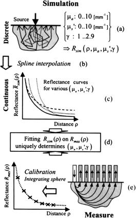
204	Methods and Algorithms for the Measurement of the Optical Parameters of Tissues

Figure 2.4 Diagram of the algorithm for the automatic spectral determination of tissue optical properties. (a) First, a set of reﬂectance curves simulated by the MC method is produced for a wide range of discrete values for each optical coefﬁcient [i.e., μa, μs, and γ = (1 − g2)/(1 − g1)]. (b) Second, the simulated curves are interpolated by cubic B-splines to provide a reﬂectance curve (c) for any value of μa, μs, and γ. Finally, for each wavelength of the spectrum, a ﬁt (d) of the measured reﬂectance curve (e) is performed onto the interpolated set of simulated curves, allowing for the determination of μa, μs, and γ. The ﬁtting

method used is the Levenberg–Marquardt algorithm.683

ranged from unity to inﬁnity, gn, where g1 is the conventional anisotropy factor, generally noted as g.

The diffusion approximation generally holds for μsρ > 5 and μs > 100μa. For shorter source-detector separations, typically when 0.5 < μsρ < 5, the second moment of the phase function g2 must also be accounted for.688 It can be shown that besides the refractive index, only three parameters are needed to accurately describe the light propagation at such small source-detector distances: μa, μs, and γ, where

γ	=	1 − g2	(2.18)
		1 − g1

Tissue Optics: Light Scattering Methods and Instruments for Medical Diagnosis

205

and γ depends on the scatterers’ relative refractive index and on the ratio between the scattering size and the wavelength; γ varies between 0.9 (Rayleigh-type scattering) and values larger than 2 (large scatterers compared to wavelength). For a Henyey-Greenstein phase function, g2 = (g1)2 and, therefore, g = g1 = γ − 1.683 The authors of Ref. 683 showed that for fractal distribution, γ is related to the fractal power of the size distribution of the scatterers.

Approximately 40 discrete values were chosen by the authors of Ref. 683 for μa and μs, ranging, respectively, from 0.003 to 10 mm−1 and from 0.5 to 10 mm−1; 20 values were chosen for γ, ranging from 1.0 to 2.9. This resulted in a fourdimensional matrix of simulated reﬂectance curves, noted as Rsim(ρi, μa, μs, γ), each coefﬁcient taking only discrete values [see Fig. 2.4(a)]. Using these parameters, 32,000 reﬂectance curves have been computed, each for a speciﬁc triplet of optical coefﬁcients (μa, μs, γ). Since the path lengths and exit positions of each simulated photon were stored, a full MC simulation was required only for each different value of γ (thus, only 20 simulations). Assuming the tissue is homogeneous, scaling relationships allow one to derive any reﬂectance curve Rsim(ρi, μa, μs, γ) from a single simulation Rsim(ρi, μa = 0, μs = 1, γ), γ being kept constant.683

Clinical measurements performed endoscopically in vivo in the stomach of human subjects were provided using the described technique and algorithm.683 The absorption and scattering properties were found to be signiﬁcantly different in the antrum and in the fundus (see Table 2.1) and were correlated with histopathologic observations.

In the six-detector ﬁber system made of 0.4-mm core diameter optical ﬁber that is described in Ref. 681, typical source-detector distances were: rsd = 0.44, 0.78, 0.92, 1.22, 1.40, and 1.84 mm. The authors performed MC simulations using a program provided by Jacques.684 In the course of their in vivo studies, temperature dependences of the absorption and the reduced scattering coefﬁcients of human forearm skin were determined (see Table 2.1).

Another six-detector ﬁber system made of 0.2-mm core diameter optical ﬁber with the following range of the source-detector separations: 0.23, 0.67, 1.12, 1.57, 2.01, and 2.46 mm, and a corresponding algorithm based on the MC simulation of light propagation and multivariate calibration models using a feed-forward artiﬁcial neural network or partial least-squares procedures were applied to the determination of optical properties in highly attenuating tissue.682 An absolute accuracy of the scattering and absorption coefﬁcients’ determination, respectively, on the level of ±2 and ±3 cm−1 (rms) was achieved. The method was applied to estimation of the optical properties of ex vivo bovine liver samples. The absorption and scat-

tering coefﬁcients, determined as μa = 14.5 ± 3.5 cm−1 and μs = 7.2 ± 3.7 cm−1 at 543 nm, and μa = 4.7 ± 1.7 cm−1 and μs = 6.7 ± 3.4 cm−1 at 633 nm, are favorably compared with the limited and varied data in the literature.

One more example of the back-reﬂectance method is tissue probing with an oblique laser beam. A simple analytical formula for the linear shift of the center of maximum diffuse reﬂection from the point of beam incidence x has been suggested to facilitate the evaluation of the optical parameters of the medium

206	Methods and Algorithms for the Measurement of the Optical Parameters of Tissues
as670,671,736
	x =	sin αi	,	(2.19)

		n(μs + 0.35μa)

where αi, is the incidence angle of the beam, n is the relative mean refractive index of the scattering medium, and μs μa. The relative index of refraction is unity for a matched boundary.

It was demonstrated that spectral dependencies of the absorption and reduced scattering coefﬁcients can be easily obtained with this method, with an accuracy of 10–17% and 5–6%, respectively.670 Oblique-incidence reﬂectometry has also been implemented with optical ﬁbers in the same way as the normal-incidence reﬂectometry described above.671 White light was delivered, and the diffusely reﬂected light was collected with a ﬁber-optic probe made from black derlin and 600-μm core diameter, low-loss optical ﬁber. The source ﬁber was oriented at a 45-deg angle of incidence, and the nine collection ﬁbers, arranged in a linear array, collected the diffusely reﬂected light. This probe was sensitive for the anisotropy in the absorption and reduced-scattering coefﬁcients, which is related to the structural anisotropy in the tissue caused, for instance, by the alignment of muscle ﬁbers. The lower absorption coefﬁcient at a 0-deg probe orientation (with respect to the muscle ﬁbers) than that at 90 deg was probably caused by the light-guiding effect of the muscle ﬁbers, which are less absorbing than the space between the muscle ﬁbers, which is occupied by blood capillaries of great absorption.736

Two precise optical systems, the ﬁber-optic spectrometer yielding spatially resolved back-reﬂectance spectra and the single-wavelength ﬁber-optic-CCD tissue imager, were used for in vivo measurements of anisotropy of scattering and absorption coefﬁcients of human skin at different body locations.692 The source-detector distances between 0.33 and 10.0 mm for 18 detecting 200-μm core diameter ﬁbers linearly aligned with a central illuminating ﬁber provided a 2D mapping of reﬂected intensity by rotation of the detecting ﬁber system around the illuminating ﬁber. A video reﬂectometry system consisted of a photometric ﬁber-coupled CCD system in direct contact with the skin, and a central optical illumination ﬁber delivering 810-nm laser light from a laser diode into the tissue. The images acquired consisted of 10242 pixels of 24 μm2. A 16-bit analog-to-digital converter was used with the CCD chip to provide the high dynamic range needed for reﬂectometry. The MC code accounting for a two-layered tissue model (skin itself and a semiinﬁnite subcutaneous fat layer) with two groups of scatterers, one of randomly distributed scatterers and another of inﬁnite dielectric cylinders (dermal collagen ﬁbers) aligned along one of the principle Cartesian axes parallel to the skin surface, was designed to evaluate scattering and absorption coefﬁcients distributions. In the skin layer, the scattering coefﬁcient was recalculated before each interaction event according to the current direction of photon propagation as692

μs = μs0[1 + f (0.5 − | cos ψ|)],

(2.20)

Tissue Optics: Light Scattering Methods and Instruments for Medical Diagnosis

207

where μs0 is a base scattering coefﬁcient, f is the fraction of scatterers oriented in the preferential direction, and ψ is the angle between the current photon direction

and the cylinder axis.

Optical coherence tomography (OCT)1,3,8,13,17,18,76,77,84,102,108–111,116,127,129,

135,139,142 is a newly developed modality that allows one to evaluate the scattering

and absorption properties of tissue in vivo within the limits of an OCT penetration depth of 1–3 mm.13,711–713,716–718,720,721 The principles and applications of OCT

are described in detail in Chapters 4 and 9. The use of OCT to measure the singlescattering coefﬁcient of tissues μs has been described by Schmitt et al. in 1993.13 In its simplest form, this method assumes that backscattered light from a tissue decreases in intensity according to720,737

=	[−	2(μa	+	]	,	(2.21)
Ib I0 exp		2(μa		μs)z	,	(2.21)

where (μa + μs) is the total attenuation of light backscattered at a depth z. For can be estimated roughly as

coefﬁcient and 2z is the round-trip distance most tissues in the NIR, μa μs; thus, μs

μs		1	(2.22)
		2z{ln[Ib(z)/I0]}
	=

or as the gradient of a graph ln[Ib(z)/I0] versus z. Experimental data for tissue OCT images show that the logarithmically scaled average for multiple indepth scans’ backscattered intensity, ln[Ib(z)], decays exponentially; thus, by performing a linear regression on this curve, the scattering coefﬁcient can be determined.13 More comprehensive algorithms accounting for multiple scattering

effects and properties of a small-angle scattering phase function are available in

the literature.711–713,716–718

Using OCT, the directional anisotropy of tissue can be studied. Thus, using an OCT system working on 1300 nm, the authors of Ref. 720, for cortical bone tissue, found changes in the scattering coefﬁcient at about 40% for a light beam perpendicular (μs = 28 cm−1) and parallel (μs = 20 cm−1) to the main direction of tissue striations. This result is qualitatively described by Eq. (2.20).

The values of absorption and scattering coefﬁcients and scattering anisotropy factor for many of the human tissues measured in vitro, ex vivo, or in vivo and calculated using the discussed and some other approaches are presented in Table 2.1.

2.7 Direct measurement of the scattering phase function

Direct measurement of the scattering phase function p(θ) is important for the choice of an adequate model for the tissue being examined.1,58,164,630,724,725 The

scattering phase function is usually determined from goniophotometric measure-

ments in relatively thin tissue samples.1,37,56,58,87,96,221,222,227,228,232,255,630,657,658,

665,666,669,719,724,725 A typical goniometer setup is depicted in Fig. 2.5. The scattering indicatrix measured with due regard for the geometry of the sample and

208	Methods and Algorithms for the Measurement of the Optical Parameters of Tissues

Figure 2.5 Schematic diagram of a goniometer for measurement of light scattering as a function of angle (scattering indicatrix measurement).255

experimental datum is approximated either by the Henyey-Greenstein phase function (HGPF)1,31,255,724,725 [see Eq. (1.15)] or by a set of HGPFs, with each function

characterizing the type of scatterers and speciﬁc contribution to the indicatrix [see Eq. (2.7)].657 In the limiting case of a two-component model of a medium con-

taining large and small (compared with the wavelength) scatterers, the indicatrix is represented in the form of anisotropic and isotropic components.56,228,658 Other

approximating functions are equally useful, e.g., those obtained from the RayleighGans approximation,228 ensuing from Mie theory,96,654,655 or a two-parameter

Gegenbauer kernel phase function (GKPF) [HGPF is a special simpler case of this phase function, see Eq. (2.8)].725 Some of these types of approximations were used to ﬁnd the dependence of the scattering anisotropy factor g for dermis and epidermis on the wavelengths in the range 300 to 1300 nm, which proved to coincide fairly well with the empirical formula37

ge gd 0.62 + λ × 0.29 × 10−3,

(2.23)

on the assumption of a 10% contribution of isotropic scattering (at least in the spectral range of 300–630 nm). The wavelength λ is given in nanometers.

Analysis of scattering indicatrices measured for sequentially stripped human-

skin-epidermal slices has demonstrated that the g value averaged over ﬁve epidermal slices is g = 0.89 ± 0.02 at λ = 633 nm.255 The measurements have been per-

formed using the setup presented in Fig. 2.5. A single-mode He:Ne laser was used as a light source. The detector was a photon-counting system based on the photomultiplier. The whole system was computer controlled. The epidermal sample was placed between a quartz slide and a hemisphere in order to avoid refraction of both incident and scattered lights. The measurements were performed in the range 0–60 deg with one-degree steps. The experimental values of the anisotropy factor g obtained using direct measurements of the scattering phase function for many types of human tissues are presented in Table 2.1.

Tissue Optics: Light Scattering Methods and Instruments for Medical Diagnosis

209

It should be noted that the correct prediction of light transport in tissues depends on the exact form of the phase function used for calculations.49,725 Sim-

ulations performed with different forms of p(θ) (HGPF, Mie, and GKPF) with the same value of cos(θ) result in the collection of signiﬁcantly different frac-

tions of the incident photons, particularly when small numerical-aperture delivery and collection ﬁbers (small source-detection separation) are employed.49,725 More

photons are collected for the distribution that has a higher probability of scattering events with θ > 125 deg. For the clinically relevant optical parameters employed in Ref. 49, the differences in light collection were more than 60%.

Moreover, for media with high anisotropy factors, precise measurements of the scattering phase function in the total angle range from 0 to 180 deg is a difﬁcult technical task that demands an extremely large dynamic range of measuring equipment. Most of the scattered radiation lies in the range from 0 to 30 deg, counting from the direction of the incident beam. In addition, measurements at angles close to 90 deg are strongly affected by scattering of higher orders, even for samples of moderate optical thickness.442

2.8 Estimates of the optical properties of human tissue

The above-discussed methods and techniques were successfully applied for estimation of optical properties of a wide number of tissues. Measurements done in vitro, ex vivo, and in vivo by different research groups are summarized in Table 2.1. Evidently, many types of animal and human tissues may have very close optical properties, but some speciﬁcity is expected. For example, normal bovine sclera is more pigmented, thicker, and its collagen structure makes it more sensitive to swelling than human sclera. Another example is porcine skin, whose epidermis structure may be quite different from human skin, particularly for aged skin. Therefore, in the Table 2.1 optical parameters of only human tissues are presented. On the other hand, human and animal tissues such as muscle, vessel wall tissue, and liver may have very similar optical properties. Thus, another reason to present only human tissues is not to overburden the table. Early published data on optical properties of both human and animal tissues are summarized in Refs. 40, 87, 691, and 696. More recent data can be found in Refs. 98, 129, 130, 164, 236–238, 263, 572, 655, 656, 672–689, 691–697, and 699–708.

Data presented in Table 2.1 reﬂect well the situation in the ﬁeld of tissue optical parameters measurements. It is clearly seen that the major attention was paid to female breast and head/brain optical properties investigations because of great importance and perspectives of optical mammography, and optical monitoring and treatment of mental diseases. Skin and underlying tissues are also well studied. Nevertheless, in general, not many data for optical transport parameters are available in the literature. Moreover, these data are dependent on the tissue preparation technique, sample storage procedure, applied measuring method and inverse problem-solving algorithm, measuring instrumentation noise, and systematic errors.

210	Methods and Algorithms for the Measurement of the Optical Parameters of Tissues

The most detailed in vitro investigations of normal and coagulated brain tissues (gray matter, white matter, cerebellum, pons, and thalamus), as well as of native tumor tissues (astrocytoma WHO grade II and meningioma), using single-integrating-sphere spectral measurements in the spectral range from 360 to 1100 nm and IMC algorithm for data processing are described in Ref. 264 (see Table 2.1). As it follows from Table 2.1, all brain tissues under study shared qualitatively similar dependencies of the optical properties on the wavelength. The scattering coefﬁcient decreased and the anisotropy factor increased with the wavelength, which can be explained by the lowering of the contribution of Rayleigh scattering and growing of the contribution of Mie scattering with the wavelength. The wavelength-dependent absorption coefﬁcient behavior of all brain tissues resembled a mixture of oxyand deoxy-hemoglobin absorption spectra. This means that in spite of careful sample preparation, it was not possible to remove all blood residuals from the tissue sections.

At the same time, the differences in the spectral characteristics of brain tissues have been observed. For example, the total attenuation coefﬁcients (μt = μa + μs) of white matter are substantially higher than those of gray matter. The two brain stem tissues (pons and thalamus) also have different optical properties. The tumors are generally macroscopically less homogeneous than any normal tissues; thus, their scattering coefﬁcients and anisotropy factors are slightly higher than those of normal gray matter. The same tendency of scattering coefﬁcients growing is typical for breast tumors (carcinomas, see Table 2.1 and Refs. 660 and 699).

After coagulation, the values of the absorption and scattering coefﬁcients increased for all tissues. The extent of this increase, however, is different for each tissue type, and is characterized by factors from 2 to 5. It was shown264 that a signiﬁcant increase of both interaction coefﬁcients is a result of substantial structure changes, caused mostly by tissue shrinkage and condensation, as well as collagen swelling and homogenization of the vessel walls. Tissue shrinkage caused by losing water at coagulation makes tissue more dense, which leads to increases of both scattering and absorption coefﬁcients in the spectral range where water absorption is weak (up to 1100–1300 nm). The refractive index microscopic redistribution of a tissue due to cellular and ﬁber proteins’ denaturation and homogenization at thermal action also may have a strong inclusion in alteration of scattering and absorption properties. The similar increase of both absorption (by a factor of 2–10) and scattering (by a factor of 2–4) coefﬁcients in the wavelength range from 500 to 1100 nm was found for coagulated human blood.

The reduced scattering coefﬁcient of skull bone is considerably less than that of brain white matter and is comparable with that of gray matter, cerebellum, and brain stem tissues. It is also comparable with scalp tissue values. At coagulation of soft brain tissues, their reduced scattering coefﬁcient may considerably exceed that of skull bone for all tissues presented in Table 2.1. This would imply that in NIR spectroscopy on the adult head, the effect of light scattering by the skull is of the same order of magnitude as that of surrounding scalp tissue and brain.719 A possible reason for this is the high values of scattering anisotropy factor g due to

Tissue Optics: Light Scattering Methods and Instruments for Medical Diagnosis

211

the speciﬁc structure of bone. For example, cortical bone consists of an underlying matrix of collagen ﬁbers, around which calcium-bearing hydroxyapatite crystals are deposited. These crystals are the major scatterers of bone;720 they are big in size and have a high refraction power, and therefore may be responsible for the high values of g. Actually, the optical properties of bone samples taken from pig skull and measured using the goniophotometric technique of thin bone slices over the wavelength range 650–950 nm gave values of anisotropy factor in the range from g = 0.925 ± 0.014 at 650 nm to g = 0.945 ± 0.013 at 950 nm, averaged for six samples.719 The corresponding values of the absorption and of the scattering coefﬁcients measured on 18 samples using the integrating sphere technique and

IMC were: μa = 0.40 ± 0.02 cm−1 and μs = 350 ± 7 cm−1 at 650 nm to μa = 0.50 ± 0.02 cm−1 and μs = 240 ± 6 cm−1.

Analyzing data received by different groups for the same brain tissue, the inﬂuence of the theoretical approach used or the sample preparation technique on results can be demonstrated. Because of a lack of experimental data for various brain tissues, at present, such a comparison can be done only for gray and white brain matter (see Table 2.1). The authors of Ref. 264, by using the IMC method for data processing of single-integrating sphere measurements, have obtained lower values for the absorption and scattering coefﬁcients than the author of Ref. 698, who used an inverse δ-Eddington method. This discrepancy may be explained by limitations of the δ-Eddington model, which is principally one-dimensional and therefore could not account for the losses of light at the side edges of the samples. This might have led to an overestimation of the extinction coefﬁcients. On the other hand, in the framework of the application of identical theoretical approaches (IMC), the usage of shock freezing and homogenization for sample preparation697 in comparison with the usage of tissue cryosections264 gives lower values of scattering coefﬁcients, at least for white brain matter. The same tendency was also demonstrated for liver samples697 and for breast tissue (compare data of Refs. 660 and 699 in Table 2.1).

The ten-sphere discrete particle model of a soft tissue indicates that the scattering coefﬁcient decreases with the wavelength approximately as μs λ2−Df for 600 ≤ λ ≤ 1400 nm, where Df is the limiting fractal dimension; 3 < Df < 4 for typical soft tissues.156 In the model of spheres ranging from 5 nm to 30,000 nm, at an interval of 5 nm, μs λ3−Df for 600 ≤ λ ≤ 1500 nm and the range of fractal dimension is 4 < Df < 5.107 Both models give the same power law for dependence of the scattering (or reduced scattering) coefﬁcient on the wavelength μs(μs) = qλ−h, with h in the range from 1 to 2 [see Eqs. (1.178)–(1.181)]. As it follows from the

data of Tables 1.5 and 2.1, most tissues such as aorta, skin, dura mater, sclera, and mucosa have parameter h = 1.16–1.62,569,570,703,704,706 which satisﬁes the model’s

predictions. The corresponding values of ﬁtting parameter q are in the range from 8.9 × 104 to 4.7 × 105 cm−1. An in vitro study of rat skin in the range from 500 to 1200 nm gave h = 1.12.571 For soft tissues, Jacques modeled the reduced scat-

tering coefﬁcient by the same power law with q ranging from 2 × 105 cm−1 to 2 × 106 cm−1 and h = 1.5.710 The experimental data for ex vivo skin samples of

212	Methods and Algorithms for the Measurement of the Optical Parameters of Tissues

Ref. 677 in the spectral range from 1000 to 2200 nm (with exclusion of dispersion of the strong water bands) are better modeled using a value q equal to 2 × 105 for h = 1.5. For the in vivo backscattering investigation of human skin and underly-

ing tissues in the wavelength range from 700 to 900 nm, constants q and h were determined as 550 ± 11 and 1.11 ± 0.08, respectively.572 The power constant h is

related to an averaged size of the scatterers; thus, once h is determined, the Mie equivalent radius aM can be derived from Eqs. (1.180) and (1.181).572 If the relative refractive index between spheres and surrounding medium is m = 1.037, the measured constant h = 1.11 leads to an aM value of 0.30 μm. Diffuse reﬂectance measurements for female breast tissues gave an aM value of 0.17 μm for normal tissue and of 0.29 μm for malignant tissue (see Table 2.1).699

In contrast to the above-discussed tissues, fat and bone tissue show very low values of the power constant: h = 0.59 for abdominal705 and h = 0.79705 or h = 0.68726 for subcutaneous fat, and h = 0.65 for bone.738,739 One of the possible

reasons for this is the speciﬁcity of fat and bone tissue structure. Fat consists mostly of fat cells; each fat cell contains a smooth drop of fat, which ﬁlls up a whole cell. Cells are spherically shaped and their diameters depend on fat content, and are in the range from 10 to 200 μm. For such big and rather homogeneous scatterers, a weak wavelength dependence of light scattering coefﬁcients might be expected. It is similar for bone, where hydroxyapatite crystals, the major scatterers, are big in size and have a high refraction power.720

Another reason for lower h is the possible inﬂuence of dispersion of lipids and water bands (see Fig. 1.5), which should decrease the inclination of the wavelength dependence in the range around 1000–1300 nm.

A decrease in h from 1.12 to 0.52 for rat skin studied in vitro in the range from 500 to 1200 nm induced by glycerol application was found.571 Because the major action of glycerol on tissue is its dehydration causes increase of tissue density, this may be a third reason for such small values of power constant h for fat and bone, being rather dense tissue and having the lowest hydration ability amongst a variety of tissues.

A low power dependence on the wavelength was also found for the scattering coefﬁcient of leg bone of the horse (only the cortical part of equine bone taken from the shaft of the third metacarpal of 2-mm thickness) measured using a singleintegrating sphere and IMC techniques.720 In the wavelength range from 520 to 960 nm, values of the scattering coefﬁcient were changed from 350 to 250 cm−1 for the constant value of g = 0.93 supposed in the calculations.

2.9 Determination of optical properties of blood

Fresh human blood placed in a calibrated thin cuvette (thickness from 0.01 to 0.5 mm, slab geometry) is usually used for the determination of blood optical parameters. Prior to the optical measurements, standard clinical tests are necessary to determine the concentration of red and white blood cells, concentration of platelets, hematocrit, mean corpuscular volume and hemoglobin, and the other

Tissue Optics: Light Scattering Methods and Instruments for Medical Diagnosis

213

parameters of interest. If blood sample oxygenation level is of interest, it may be controlled using a conventional blood gas analyzer.164 In most cases, the ex-

periments are performed with either completely oxygenated or completely deoxygenated blood.48,164,724,729,730 To obtain complete oxygen saturation, the sample is exposed to air or O2.48,164 To completely deoxygenate the blood, sodium dithionite (Na2S2O4) is added.164 To be sure that neither the volume nor the surface area of

the blood particles changes during the experiments, the pH of the samples should be maintained in the range of physiological values, at approximately 7.4.

In reality, blood is ﬂowing through the blood vessels and it is therefore preferable to study the optical properties of ﬂowing blood. The RBCs in ﬂow are subject to deformation and orientation. At lower shear rates, reversible aggregation occurs; while under the higher shear rates, erythrocytes are deformed into ellipsoids. The experiments with ﬂowing undiluted and diluted blood are reported in Refs. 48, 49 and 689. Roggan et al.48 have assembled sophisticated equipment to analyze the inﬂuence of different hematocrit, ﬂow velocity, osmolarity, hemolysis, and oxygen saturation on the optical properties of RBC suspensions submerged in a saline solution. Nilsson et al.49 investigated the inﬂuence of slow heating on the optical properties of whole ﬂowing blood. The inﬂuence of the shear stress on the opti-

cal properties of whole completely oxygenated blood was studied by Steenbergen et al.689

Several authors reported the values of the optical parameters of blood determined from the single scattering experiments (Table 2.2). Reynolds et al.740 determined values of the absorption cross section, the scattering cross section, and the anisotropy factor of blood for a number of wavelengths in the visible and nearinfrared spectral range, and compared the experimental values with the calculated (Mie theory) ones. In Mie calculations, they used the value of 2.79 μm for the

RBC radius, and the value of 1.036 for the RBC refractive index (relative to blood plasma).183,740

Flock et al.690 measured the total attenuation coefﬁcient and the scattering phase function of a diluted whole blood sample [phosphate buffered saline solution (PBS), hematocrit (Hct) of 1%, cuvette < 100-μm thick] at a wavelength of 632.8 nm.

Steinke and Shepherd741 determined the total attenuation coefﬁcients, the scattering cross sections and the anisotropy factors of RBCs suspended in blood plasma and in PBS (0.9%) from the collimated transmittance and scattering phase function measurements for a wavelength of 632.8 nm, and from the calculations using Mie theory. For measurements of collimated transmittance, cuvettes with a thickness of 144 μm (slab geometry) were used. For the goniometrical measurements, an

American Optical Hemoglobinometer cuvette (path length 51 μm) was employed. Yaroslavsky et al.164,724 measured the scattering phase functions of diluted

whole blood samples; approximated the experimental scattering phase functions using Mie theory, Henyey-Greenstein (HGPF), or Gegenbauer kernel (GKPF) functions [see Eqs. (1.15), (2.7), (2.8), and (2.10)]; and determined the anisotropy factors for each approximation at a wavelength of 633 nm. For Mie calculations,

Table 2.2 Optical parameters of blood determined and approximated from the single scattering experiments (S—oxygen saturation, Hct— hematocrit, aRBC—radius of RBC, mRBC—relative index of refraction of RBC, lcuv—cuvette thickness).725

λ,	S,	σa,	σs,	σt,	μt,
nm	%	μm2	μm2	μm2	cm−1	g	Phase function	Condition	Ref.

665	100	0.060	57.20	7.47	0.9951
675	100	0.060	56.14	7.44	0.9950
685	100	0.059	55.09	7.39	0.9949
955	100	0.191	33.47	6.66	0.9925
960	100	0.187	33.18	6.66	0.9924
965	100	0.185	32.90	6.65	0.9924
665	0	0.542	56.58	7.38	0.9951
675	0	0.535	55.53	7.35	0.9950
685	0	0.484	54.56	7.31	0.9949
955	0	0.090	33.54	6.68	0.9925
960	0	0.085	33.27	6.67	0.9924
965	0	0.080	32.98	6.66	0.9924
630	100	0.099	56.37
660	100	0.066	54.20
685	100	0.063	53.53
800	100	0.131	42.24
632.8	100			29	0.974
632.8
	100		63.82	7.09	0.9853
	100		66.62	7.40	0.9948
	100		81.24	9.03	0.9818
	100		79.27	8.81	0.9926

Mie	Comparison with Mie theory;
	aRBC = 2.79 μm; mRBC = 1.036	740

Experiment

HGPF	Hct = 1%; lcuv < 100 μm	690
Mie	lcuv = 144 μm and 51 μm	741
	RBC in plasma

RBC in PBS (0.9%)

214

Tissues of Parameters Optical the of Measurement the for Algorithms and Methods

Table 2.2 (Continued).

λ,	S,	σa,	σs,	σt,	μt,
nm	%	μm2	μm2	μm2	cm−1	g	Phase function	Condition	Ref.
632.8	100					0.982	HGPF	(α = 1.82)	724
	100					0.995	GKPF	(α = 1.82)
632.8								Hct = 0.1%; pH = 7.4;	164
	100					0.971	HGPF	lcuv = 10 μm
	100					0.997	GKPF	(α = 3.658)
	100					0.996	Mie	aRBC = 2.995 μm, mRBC = 1.04
577				≈95				Hct = 1%; pH = 7.4; lcuv = 100	730
	100			≈95		0.966	HGPF	and 10 μm
	100					0.997	GKPF	(α = 1.5)
	100					0.997	Mie
	100					0.9995	Rayleigh-Gans

Diagnosis Medical for Instruments and Methods Scattering Light Optics: Tissue

215

216	Methods and Algorithms for the Measurement of the Optical Parameters of Tissues

the RBC radius was assumed to be equal to 2.995 μm, and the RBC refractive index equal to 1.04 (relative to PBS). The scattering phase functions were measured in the angle range from 2 to 18 deg. For the experiments, fresh samples of whole blood were collected into heparinized containers and diluted with a phosphate buffer solution (pH = 7.4) to a Hct = 0.1%. The diluted blood samples were placed into the cuvettes (10-μm thick, slab geometry).

Hammer et al.730 presented a comprehensive study of RBC single scattering behavior. The authors measured the collimated transmittance and the scattering phase functions of the RBC suspensions in isotonic PBS (pH = 7.4, Hct = 1%) for a number of wavelengths in the visible spectral range from 458 to 660 nm. The scattering phase functions were measured for 20 scattering angles in the range between 0.75 and 14.5 deg. For the transmission measurements, a cuvette with a thickness of 100 μm (slab geometry), and for the scattering phase function measurements, a cuvette with a thickness of 10 μm (slab geometry) were used.

The optical properties of the diluted and whole human blood, determined using indirect techniques, were reported by Yaroslavsky et al.,164,724 Nilsson et al.,49

Roggan et al.,48 and Steenbergen et al.689 A summary of the optical properties of diluted and whole blood determined using indirect techniques is given in Table 2.3.

The optical parameters of completely oxygenated whole blood samples were determined on a selected wavelength of 633 nm164 and in the near-infrared spectral range724 from double integrating sphere measurements using an inverse Monte Carlo technique (see Table 2.3). The measured values included the diffuse reﬂectance, the total transmittance, and the collimated transmittance. From the measured data, the absorption coefﬁcient, the scattering coefﬁcient, and the anisotropy factor (under the assumption of the Henyey-Greenstein phase function) were derived. In Ref. 164, blood samples with Hct = 38% and oxygen saturation S > 98% were studied. In Ref. 724, the spectral range investigated extended from 700 to 1200 nm and blood samples with Hct = 45.5 ± 0.5% placed into calibrated cuvettes (thickness 0.1 and 0.5 mm, slab geometry) were used. The spectral dependences of the optical parameters of whole blood obtained in Ref. 409 are pre-

sented in Fig. 2.6. In addition, the effect of the scattering phase function approximation on the resulting estimates of the optical parameters was analyzed.164,724

The Henyey-Greenstein, Gegenbauer kernel, or Mie phase functions were considered [see Eqs. (1.15), (2.7), (2.8), and (2.10)]. The calculated angular distributions of scattered light were compared with goniophotometric measurements performed at a wavelength of 633 nm. The scattering phase functions of highly diluted blood samples (Hct = 0.1%, S > 98%) were also measured using a goniophotometer. To evaluate the obtained data, the angular distributions of scattered light for optically thick samples were calculated and the results were compared with goniophotometric measurements. The data presented have shown that the employed approximation of the scattering phase function can have a substantial impact on the derived values of μs and g, while μa and the reduced scattering coefﬁcient μs are much less sensitive to the exact form of the scattering phase function. It was shown that both Rd and Tt are strongly affected by the form of the phase function, and that

Table 2.3 Overview of the optical properties of blood ( data taken from the graphs of the respective reference; Hct—hematocrit, S—oxygen saturation, aRBC—radius of RBC, mRBC—relative index of refraction of RBC, tb—blood temperature, vsh—shear rate, lcuv—cuvette thickness).725

λ,	μa,	μs,	μt,		μs,	Phase
nm	cm−1	cm−1	cm−1	g	cm−1	function	Conditions	Ref.
633	15.5	645	–	0.982	11.6	HGPF	Hct = 45%, S > 98%	724
	15.4	2239	–	0.995	11.2	GKPF	α = 1.82
633	15.2 ± 0.6	400 ± 30	–	0.971 ± 0.001	11.7 ± 1.2	HGPF	Hct = 38%, S > 98%	164
	16.1 ± 0.6	4130 ± 170		0.997 ± 0.0001	12.4 ± 0.9		7 samples
	16.1 ± 0.6	4130 ± 170	–	0.997 ± 0.0001	12.4 ± 0.9	GKPF	α = 3.658
	16.3 ± 0.5	2390 ± 160	–	0.9962 ± 0.0001		Mie	aRBC = 2.995 μm
							mRBC = 1.04
633						HGPF	Hct = 44 ± 3%, S = 100%	49*
	3.0	–	–	–	18.5		tb = 25◦C
	3.5	–	–	–	18.2		tb = 35◦C
	4.0	–	–	–	18.0		tb = 42◦C
	4.5	–	–	–	21.0		tb = 48◦C
	6.0	–	–	–	17.0		tb = 54◦C
633						GKPF	α = 1.0; Hct = 41%	48*
	20	–	–	–	20		S = 25%
	16	–	–	–	20		S = 50%
	12	–	–	–	20		S = 75%
	7	–	–	–	18		S = 100%
							α > 0.99, Hct = 5%
	1.25	300					S = 0%
	1.10	300					S = 100%
633						HGPF	Hct = 50 ± 0.5%	689*
							S = 100%
	–	–	–	–	–	0.950–0.963	vsh = 50 s−1
	–	–	–	–	–	0.956–0.965	vsh = 100 s−1

Diagnosis Medical for Instruments and Methods Scattering Light Optics: Tissue

217

Table 2.3 (Continued).

λ,

μa,

μs,

−1

μt,

−1

Phase

−1

function

Conditions

Ref.

–

≈1200

–

0.960–0.966

vsh = 150 s−1

–

≈1200

–

0.962–0.967

vsh = 200 s−1

–

≈1200

–

0.963–0.968

vsh = 300 s−1

–

≈1200

–

0.963–0.970

vsh = 400 s−1

–

≈1200

–

0.964–0.973

vsh = 500 s−1

488

102.2

134.4

–

0.91

IAD, HGPF, lcuv = 90 μm

742

218

Tissues of Parameters Optical the of Measurement the for Algorithms and Methods

Tissue Optics: Light Scattering Methods and Instruments for Medical Diagnosis

219

(a)

(b)

(c)

Figure 2.6 Optical properties of whole blood.724,725 Hematocrit, Hct = 45.5 ± 0.5%; oxygen saturation, S > 98%. Average of six samples. Bars are standard errors. (a) Absorption coefﬁcient, (b) scattering coefﬁcient, (c) anisotropy factor.

220	Methods and Algorithms for the Measurement of the Optical Parameters of Tissues

the magnitude of this inﬂuence depends on the thickness of the blood sample. The presented data prove that the variations of the employed scattering phase function approximation can cause large discrepancies in the derived optical parameters. Therefore, the exact knowledge of the scattering phase function is required for the precise determination of the blood optical constants.

Nilsson et al.49 studied the inﬂuence of slow heating on the optical properties of completely oxygenated whole blood at a wavelength of 633 nm (Table 2.3). The diffuse reﬂectance, the total transmittance, and the collimated transmittance were measured at different temperatures using a double integrating sphere technique. The absorption coefﬁcient, the scattering coefﬁcient, and the anisotropy factor (assuming the Henyey-Greenstein phase function) were determined using an inverse adding-doubling method. For the measurements, whole blood was collected into tubes that contained ethylenediaminetetraacetic acid (EDTA) to prevent coagulation. The hematocrit of the investigated samples was 44 ± 3%. During the measurements, the blood was pumped at a ﬂow rate of 10.7 ml/min. The ﬂow cell (length = 65 mm, height = 34 mm, total thickness = 2.5 mm) was placed between the integrating spheres. The blood sample thickness in the ﬂow cell was 0.48 ± 0.02 mm. The blood was heated from approximately 25 to 55◦C at rates between 0.2 and 1.1◦C/min. While the blood was heated, the integrating sphere measurements were continuously taken. The authors found that changes in optical properties of blood due to slow heating were reversible until a temperature of 44.6–46.6◦C. Coagulation of blood occurred at approximately 55◦C.

One of the most extensive studies of the macroscopic optical properties of RBC suspension at different physiological and biochemical conditions (hematocrit, oxygen saturation, ﬂow velocity, osmolarity, and hemolysis) were done by Roggan et al. (Table 2.3).48 The authors measured the optical parameters of RBCs suspended in PBS under ﬂow conditions using a double integrating sphere technique and determined optical coefﬁcients using an inverse Monte Carlo method. The absorption coefﬁcient, the scattering coefﬁcient, and the anisotropy factor (assuming Gegenbauer kernel phase function with α = 1) were determined for the oxygenated and deoxygenated RBC suspensions (Hct = 5%) under normal physiological conditions (see Fig. 2.7). For the experiments, erythrocytes were separated from the blood plasma and white cell fraction, washed in PBS (300 mosmol/l, pH = 7.4), and suspended in the PBS. The hematocrit was adjusted by diluting the erythrocytes with PBS. By using PBSs with different osmolarities, the osmolarity of the RBC suspension was varied. Hemolysis was induced by diluting the suspensions with distilled water. Blood oxygenation and circulation was adjusted and controlled using an extracorporal circulation unit. Blood temperature was kept constant at 20◦C. The thickness of the ﬂow-through cuvette was 97 μm.

Roggan et al.48 have also come to the conclusion that an accurate approximation of the scattering phase function plays an important role in the correct determination of the optical properties of blood. It was found that absorption and scattering increased linearly with hematocrit (for Hct < 50%). Absorption and scattering decreased slightly with an increase of shear rate. Among the ﬂow parameters, axial

Tissue Optics: Light Scattering Methods and Instruments for Medical Diagnosis

221

Figure 2.7 Optical properties of RBCs suspended in PBS (Hct = 5%, osmolarity = 300 mosmol/l, shear rate = 500 s−1).48

migration was the main factor that inﬂuenced optical properties. Deformation of the erythrocytes had no impact on optical properties if the volume and hemoglobin content of the RBCs were kept constant. Hemoglobin solutions had a smaller absorption than RBC suspensions with the same concentration of hemoglobin. Obviously, the change in oxygenation of RBC suspensions induced the expected change in the absorption coefﬁcient. The scattering coefﬁcient was not affected by the change in the oxygenation of erythrocytes. The spectral dependences of the optical parameters of RBCs suspended in a PBS (Hct = 5%, shear rate = 500 s−1, osmolarity = 300 mosmol/l) are given in Fig. 2.7.

Steenbergen et al.689 analyzed the effect of shear rate on the optical properties of the completely oxygenated whole blood (Table 2.3). The collimated transmission and the angular distributions of light intensity were measured at 633 nm for

222	Methods and Algorithms for the Measurement of the Optical Parameters of Tissues

various shear rates (from 50 to 500 s−1) and blood layer thicknesses (from 20 to 100 μm). For shear rates above 150 s−1, the total attenuation coefﬁcient was determined directly from the collimated transmission measurements. The anisotropy factor was determined from the angular intensity distributions using an inverse Monte Carlo technique and assuming the Henyey-Greenstein scattering phase function. The value of the total attenuation coefﬁcient (μt = 1200 cm−1) was determined from the collimated transmittance measurements, and the values of the absorption coefﬁcient (μa = 7 and 10 cm−1) were taken from the literature.48 In addition, the authors measured the anisotropy g-factor for blood layers with different thicknesses and determined the actual g-factor by extrapolating their results to the layer thickness of zero. The hematocrit of the investigated blood varied between 49.5 and 50.5%. A continuous increase of the g-factor (from 0.950 to 0.973) with an increase of shear rate was found.

The optical properties of blood-perfused tissues are signiﬁcantly affected by tissue blood content. This is caused by two factors: ﬁrst, the optical properties of whole blood itself are substantially different from those of soft tissues; and second, whole blood is an extremely turbid medium with an extraordinary high scattering anisotropy (see Tables 2.2 and 2.3). Thus, it has a very short optical mean free path and a very long transport mean free path compared to the majority of bloodless tissues. As a result, the presence of even a small amount of blood greatly changes the process of light propagation in tissues. This point is illustrated

by Fig. 2.8, where the transport mean free path has been calculated for bloodless tissues and blood-containing brain tissues at two wavelengths.666,725 Optical prop-

erties of other blood-containing tissues are affected in a similar manner. As a result, the optical response of tissue depends strongly on the presence of blood and on its relevant parameters such as oxygen saturation and hematocrit. This opens wide possibilities for optical diagnostics, but also makes the dosimetry of light in tissues

a more difﬁcult task.

Laser photodynamic therapy19,26,29,35 and laser-induced interstitial thermal therapy (LITT) of deep tumors2 are the most promising techniques among the least invasive therapies of cancer. In this case, besides the knowledge of the optical properties of tumor tissue and the surrounding substances, the knowledge of the blood content and its optical properties is essential for therapy planning and for exact dosimetry. In addition, knowledge of the optical properties of tissues and blood allows one to determine the most effective treatment wavelength, where the penetration depth of laser light is maximal. This emphasizes the need for an explicit account of the blood content in the modeling of laser-tissue interaction—for example, the planning of clinical procedures such as LITT or photodynamic therapy.

2.10Measurements of tissue penetration depth and light dosimetry

In practice, the direct measurements of the penetration depth of various tissues at different wavelengths or at some speciﬁc wavelength are valuable. In partic-

Tissue Optics: Light Scattering Methods and Instruments for Medical Diagnosis

223

Figure 2.8 Transport mean free path [lt = (μa + μs)−1] at the wavelengths of 800 and 1100 nm for white brain matter (WM), gray brain matter (GM), oxygenated blood, deoxygenated blood, perfused white matter, and perfused gray matter.725 These are based on the results of Refs. 48 and 666. A blood hematocrit of 40% was assumed in computing the data for perfused tissues. CBV—cerebral blood volume.

ular, such data allow one to provide a strategy of laser phototherapy. As shown earlier, a detailed calculation of light distribution in tissues can be very complex and frequently requires numerical solutions of the radiative transfer equation, Eq. (1.9). However, if a speciﬁc experimental arrangement is provided, i.e., a “wide” beam irradiation of “semi-inﬁnite” samples, and light is scattered into a practically isotropic distribution very close to the irradiated surface, the onedimensional diffusion model may be used, which gives the solution described by Eq. (1.30) valid for the depths z ≥ 2ld = 2/μeff, where μeff is deﬁned by Eq. (1.18).

Using an analog of Eq. (1.30) and providing measurements within thick tissue slabs at irradiation by a parallel laser beam 5-cm wide (at one of the wavelengths 633, 675, 780, or 835 nm) and light detecting by the measuring needle with an optic ﬁber inserted into a tissue sample, values of penetration depth were estimated for a number of normal and pathological tissues.693 These data are summarized in Table 2.4. It should be noted that from the performed measurements, ld = 1/μeff was determined. The detecting ﬁber tip captures an equal proportion of the ﬂuence rate of light at every point from z ≥ 2ld to greater tissue depths. Logarithmizing the detector response as a function of the position of the needle, z, and using the method of least squares, a ﬁtted straight line was obtained, whose slope is the effective attenuation coefﬁcient μeff = 1/ ld [see Eq. (1.30)].

Table 2.4 Optical penetration depth of tissues ld in millimeters measured ex vivo for a few wavelengths. The number of samples from different bodies measured for each tissue is given in brackets (a standard error and babsolute mean deviation, for others error obtained by the method of least squares is presented).693

Tissue	ld, mm	ld, mm	ld, mm	ld, mm
	λ = 633 nm	λ = 675 nm	λ = 780 nm	λ = 835 nm
Blood	0.19 ± 0.01a (10)	0.28 ± 0.01a (10)	0.42 ± 0.02a (10)	0.51 ± 0.02a (10)
Sarcomas	0.2–4.0 (10)	0.4–4.3 (6)	0.5–4.6 (6)	–
Liver (cirrhosis)	0.43 ± 0.06b (5)	0.60 ± 0.02 (2)	1.04 ± 0.02 (2)	–
	–	0.58 ± 0.01	0.99 ± 0.02	–
Spleen	0.49 ± 0.07b (5)	0.87 ± 0.02 (2)	1.21 ± 0.01 (2)	–
	–	0.94 ± 0.01	1.16 ± 0.02	–
Parotid gland	0.61 ± 0.08b (3)	–	–	–
Bronchial ganglion metastasis	1.05 ± 0.01 (2)	–	–	–
	1.01 ± 0.01	–	–	–
Lung	0.81 ± 0.06a (10)	1.09 ± 0.11b (4)	1.86 ± 0.12b (4)	2.47 ± 0.03 (1)
Bronchial cyst	1.05 ± 0.02 (2)	–	–	–
	0.97 ± 0.02	–	–	–
Cloquet ganglion metastasis	1.12 ± 0.01 (1)	–	–	–
Thyroid gland	1.23 ± 0.08a (15)	1.42 ± 0.15b (5)	1.70 ± 0.16b (5)	3.04 ± 0.05 (1)
Neurilemoma	1.23 ± 0.02 (1)	–	–	–
Pelvic ganglion	1.39 ± 0.11b (6)	1.42 ± 0.01 (2)	1.83 ± 0.02 (2)	2.32 ± 0.03 (1)
	–	1.45 ± 0.02	1.78 ± 0.02	–
Aggressive ﬁbromatosis	1.41 ± 0.16b (4)	1.54 ± 0.03 (2)	1.87 ± 0.02 (2)	–
	–	1.44 ± 0.03	1.77 ± 0.03	–
Hepatic metastasis	1.53 ± 0.15b (5)	1.81 ± 0.21b (3)	2.48 ± 0.30b (3)	3.27 ± 0.03 (2)
	–	–	–	3.81 ± 0.03
Lung carcinoma	1.68 ± 0.15b (7)	2.01 ± 0.27b (3)	2.82 ± 0.31b (3)	3.89 ± 0.03 (1)
Prelaryngeal striated muscle	1.72 ± 0.20b (3)	–	–	–

224

Tissues of Parameters Optical the of Measurement the for Algorithms and Methods

Table 2.4 (Continued).

Tissue	ld, mm			ld, mm	ld, mm	ld, mm
	λ = 633 nm			λ = 675 nm	λ = 780 nm	λ = 835 nm
Mammary fat	1.81 ±		0.09a (10)	2.03 ± 0.18b (6)	2.24 ± 0.19b (6)	2.79 ± 0.28b (3)
Mammary tissue	2.59 ±		0.18a (14)	2.87 ± 0.30b (5)	3.12 ± 0.32b (5)	3.54 ± 0.40b (3)
Mammary displasia	2.21 ±		0.20b (9)	2.68 ± 0.29b (3)	3.03 ± 0.33b (3)	–
Mammary carcinoma	2.87 ±		0.22a (10)	3.14 ± 0.36b (3)	3.62 ± 0.41b (3)	4.23 ± 0.04 (1)
Uterine mioma	2.74 ±		0.22b (6)	2.93 ± 0.03 (1)	3.28 ± 0.03 (1)	–
Uterus	2.14 ±		0.18a (15)	2.40 ± 0.22b (4)	2.61 ± 0.25b (4)	3.31 ± 0.02 (1)
Submaxillary gland	2.49 ±		0.23b (3)	–	–	–
Malignant ﬁbrous histiositoma	2.48 ±		0.03 (1)	–	–	–
Colon	2.48 ±		0.21b (7)	2.73 ± 0.29b (3)	2.91 ± 0.31b (3)	–
Lipoma	2.83 ±		0.21a (11)	3.03 ± 0.29b (4)	3.71 ± 0.33b (4)	4.19 ± 0.03 (1)
Mesenquinoma	4.01 ±		0.03 (1)	–	–	–
Axillar epidermoid carcinoma	2.12	±	0.18b (8)	2.51 ± 0.22b (4)	2.64 ± 0.23b (4)	3.24 ± 0.03 (1)
Liver (postmortem)	1.20	±	0.13a (10)	1.69 ± 0.16a (10)	2.91 ± 0.30a (10)	3.68 ± 0.35a (10)
Brain (postmortem)	0.92	±	0.08a (10)	1.38 ± 0.13a (10)	2.17 ± 0.16a (10)	2.52 ± 0.19a (10)
Muscle (postmortem)	1.47	±	0.10a (10)	1.63 ± 0.10a (10)	3.46 ± 0.23a (10)	3.72 ± 0.29a (10)

Diagnosis Medical for Instruments and Methods Scattering Light Optics: Tissue

225

226	Methods and Algorithms for the Measurement of the Optical Parameters of Tissues
The	quantity usually measured in dosimetry is the irradiance F (r¯)	[see
			694
Eq. (1.11)], which is deﬁned as the power per receiving area of a ﬂat detector.

For this deﬁnition, light entering differently from perpendicular incidence contributes with reduced impact and light from below does not contribute at all. Lightinduced tissue heating or any photobiological effect in tissue or cells depends on light absorption. For isotropic media, absorption is not sensitive to the angle of irradiation; thus, an adequate light dosimetric quantity should be the total radi-

ant energy ﬂuence rate U (r¯) [see Eq. (1.12)] or the space irradiance,	694	For an
the light power hitting a sphere divided by the sphere’s cross section.		For an

deﬁned as

isotropic space distribution of light intensity, the space irradiance is four times the irradiance measured for the same point within the tissue (r¯).

In Ref. 694, experimental data for the diffuse reﬂectance Rd and the collimated transmission Tc of an isolated bone specimen with a deﬁned thickness d were used for the MC calculation of the transmitted irradiance F (d) and its comparison with the space irradiance at the same point U (d) inside a specimen of inﬁnite thickness. Finally, the dosimetric correction factor U/F was evaluated. The results of dosimetric correction using in vitro experimental data and corresponding calculated data for human skull bone are presented in Table 2.5. The calculations of the absorption coefﬁcient μa and the reduced scattering coefﬁcient μs from the measured

Rd and Tc were performed by a simpliﬁed procedure valid for a thickness d of the

bone with μeffd > 2. In this case, Tc = Tceff exp(−μeffd). As shown in Ref. 694, in good approximation, Tceff, Rd, and U/F depend only on the ratio μa/μs. The

knowledge of Tceff allows one to evaluate μeff from the equation for Tc and, furthermore, μa and μs from Eq. (1.18) and the known ratio μa/μs. All MC calculations were done for a tissue index of refraction n¯ = 1.35 and anisotropy factor g = 0.8.

2.11 Refractive index measurements

The mean refractive index n¯ of a tissue is deﬁned by the refractive indices of its scattering centers material ns and ground (surrounding) matter n0 [see Eqs. (1.150)–(1.154)]. The refractive index variation in tissues, quantiﬁed by the ratio m ≡ ns/n0, determines light scattering efﬁciency. For example, in a simple monodisperse tissue model, such as dielectric spheres of equal diameter 2a, the reduced scattering coefﬁcient is179

	≡ μs(1 − g) = 3.28πa2ρs	2	π		0.37
μs	≡ μs(1 − g) = 3.28πa2ρs	2	λa		(m − 1)2.09,	(2.24)

where μs = σscaρs is the scattering coefﬁcient, σsca is the scattering cross section, ρs is the volume density of the spheres, g is the scattering anisotropy factor, and λ is the light wavelength in the scattering medium. This equation is valid for noninteracting Mie scatterers g > 0.9, 5 < 2πa/λ < 50, and 1 < m < 1.1.

For example, epithelial nuclei can be considered as spheroidal Mie scatters with refractive index, nnc, that is higher than that of the surrounding cytoplasm, ncp. Normal nuclei have a characteristic diameter of d = 4–7 μm. In contrast, dysplastic

Table 2.5 Optical properties and dosimetric correction factor U/F of skull bone for different wavelengths (values are presented as mean ± SEM; to obtain the space irradiance U in an intact cochlea transmitted irradiance measured for specimen slabs have to be multiplied by U/F ).694

λ, nm	μa/μs	Tceff	μa, cm−1	μs, cm−1	μeff, cm−1	U/F
593	0.0135 ± 0.0048	0.585 ± 0.054	0.561 ± 0.108	47.1 ±8.3	8.70 ± 0.91	10.0 ±1.5
635	0.0072 ± 0.0018	0.501 ± 0.038	0.371 ± 0.022	55.7 ±9.1	7.80 ± 0.44	12.9 ±1.4
690	0.0035 ± 0.0008	0.398 ± 0.026	0.169 ± 0.011	51.1 ±7.3	5.04 ± 0.32	17.7 ±1.7
780	0.0028 ± 0.0005	0.367 ± 0.026	0.107 ± 0.009	40.0 ±4.6	3.56 ± 0.18	19.5 ±1.6
830	0.0028 ± 0.0005	0.367 ± 0.027	0.104 ± 0.009	38.8 ±4.4	3.45 ± 0.16	19.4 ±1.6

Diagnosis Medical for Instruments and Methods Scattering Light Optics: Tissue

227

228	Methods and Algorithms for the Measurement of the Optical Parameters of Tissues

nuclei can be as large as 20 μm, occupying almost the entire cell volume.620 In the

visible range, where the wavelength λ0 d, the Van de Hulst approximation can be used to describe the elastic scattering cross section of the nuclei as180,181

σsca(λ, d) =	2	πd2	1 −	δ	+	2	δ	2	,	(2.25)

	1			2 sin δ			sin δ

where δ = 2πd(nnc − ncp)/λ0; λ0 is the wavelength of the light in vacuum. This expression reveals a component of the scattering cross section, which varies periodically with inverse wavelength. This, in turn, gives rise to a periodic component in the tissue optical reﬂectance. Since the frequency of this variation (in inverse wavelength space) is proportional to particle size, the nuclear size distribution can be obtained from the Fourier transform of the periodic component.

Measuring refractive indices in tissues and their constituent components is an important focus of interest in tissue optics because the index of refraction determines light reﬂection and refraction at the interfaces between air and tissue, detecting ﬁber and tissue, and tissue layers; it also strongly inﬂuences light propagation

and distribution within tissues, deﬁnes the speed of light in tissue, and governs how

the photons migrate.31,129,130,175,178,206,743,677,712,713,744–754 Although these stud-

ies have a rather long history,87 the mean values of refractive indices for many tissues are missing in the literature. According to Ref. 87, most of them have refractive indices for visible light in the 1.335–1.620 range (e.g., 1.55 in the stratum corneum, 1.620 in enamel, and 1.386 at the lens surface). It is worthwhile noting that in vitro and in vivo measurements may differ signiﬁcantly. For example, the refractive index in rat mesenteric tissue in vitro was found to be 1.52 compared with only 1.38 in vivo.87 This difference can be accounted for by the decreased refractivity of ground matter, n0, due to impaired hydration.

Indeed, the optical properties of tissues, including refractive indices, are known to depend on water content. The refractive indices of water over a broad wavelength range from 200 nm to 200 μm have been reported in Ref. 87. Speciﬁcally, nw = 1.396 for λ = 200 nm, 1.335 for λ = 500 nm, 1.142 for λ = 2,800 nm, 1.400 for λ = 3,500 nm, 1.218 for λ = 10,000 nm, and 2.130 for λ = 200 μm. Equation (1.202) was shown to be valid for pure water in the visible and NIR wavelength ranges corresponding to the best light transmission through tissues.630

To model tissue by a mixture of water and a bioorganic compound of a tissue is more adequate. For instance, the refractive index of human skin can be approximated by a 70/30 mixture of water and protein.677 Assuming that protein has a constant refractive index value of 1.5 over the entire wavelength range, the authors of Ref. 677 have suggested the following expression for estimation of skin index of refraction:

nskin(λ) = 0.7(1.58 − 8.45 × 10−4λ + 1.10 × 10−6λ2 − 7.19 × 10−10λ3

+ 2.32 × 10−13λ4 − 2.98 × 10−17λ5) + 0.3 × 1.5,

(2.26)

where wavelength λ is in nanometers.

Tissue Optics: Light Scattering Methods and Instruments for Medical Diagnosis

229

For different parts of a biological cell, values of refractive index in the NIR range can be estimated as follows: extracellular ﬂuid, n¯ = 1.35–1.36; cytoplasm, 1.360–1.375; cell membrane, 1.46; nucleus, 1.38–1.41; mitochondria and organelles, 1.38–1.41; melanin, 1.6–1.7.58 Scattering arises from mismatches in refractive index of the components that make up the cell. Organelles and subcomponents of organelles having indices different from their surroundings are expected to be the primary sources of cellular scattering. The cell itself may be a signif-

icant source of small-angle scatter in applications like ﬂow cytometry in which cells are studied separately.145,149 In contrast, in tissues where cells are surrounded

by other cells or tissue structures of similar index, certain organelles become the important scatterers. For instance, the nucleus is a signiﬁcant scatterer because it

is often the largest organelle in the cell and its size increases relative to the rest of the cell throughout neoplastic progression.150–153,163,166,170,180,704 Mitochon-

dria (0.5–1.5 μm in diameter), lysosomes (0.5 μm), and peroxisomes (0.5 μm) are very important scatterers whose size relative to the wavelength of light suggests that they must make a signiﬁcant contribution to backscattering. Granular melanin, traditionally thought of as an absorber, must be considered an important scatterer because of its size and high refractive index.58 Structures consisting of membrane layers, such as the endoplasmic reticulum or Golgi apparatus, may prove signiﬁcant because they contain index ﬂuctuations of high spatial frequency and amplitude. Besides cell components, ﬁbrous tissue structures such as collagen and elastin must be considered as important scatterers.

Refractivity measurements in a number of strongly scattering tissues at 633 nm performed with a ﬁber-optic refractometer are schematically shown in Fig. 2.9.178

Figure 2.9 Schematic of experimental setup for determining the index of refraction. A bare quartz ﬁber is placed in a cladding of the substance to be measured. The angular light output distribution is measured, and the index is determined from Eq. (2.27).178

230	Methods and Algorithms for the Measurement of the Optical Parameters of Tissues

The method is based on a simple concept: that the cone of light issuing from an optical ﬁber is dependent on the indices of the cladding material, core material (quartz), and air into which the cone of light emerges. The cladding on a 1-mm core diameter optical ﬁber was stripped from the ﬁber, and the tissue for which the index is to be measured was substituted for the cladding. With the index for air (n0) and the quartz ﬁber (nq) known, along with the emitted angular light distribution (θ) measured at the optical ﬁber’s output, the following equation for the determination of tissue index of refraction (n¯ ) can be derived from the expression for the ﬁber numerical aperture:178

2	− [n0 sin θ]	2	-	1/2	.	(2.27)
n¯ = ,nq

Using this simple and sensitive technique, it was found that fatty tissue has the largest refractive index (1.455), followed by kidney (1.418), muscular tissue (1.410), and then blood and spleen (1.400).178 The lowest refractive indices were found in lungs and liver (1.380 and 1.368, respectively).178 Also, it turned out that tissue homogenization does not signiﬁcantly affect the refractive indices (the change does not exceed a measurement error equal to 0.006), whereas coagulated tissues have higher refractive indices than native ones (for example, for egg white, n¯ changing from 1.321 to 1.388). Moreover, there is a tendency for refractive indices to decrease with increasing light wavelength from 390 to 700 nm (for example, for bovine muscle in the limits 1.42 to 1.39), which is characteristic of the majority of related abiological materials.

Experimental values of the mean refractive index for some tissues measured for selected wavelengths are summarized in Table 2.6.

The principle of total internal reﬂection at laser beam irradiation is also used for tissue and blood refraction measurements.746,747 The schematic of a laser re-

fractometer is shown in Fig. 2.10.746 A thin tissue sample is sandwiched between two right-angled prisms that are made of ZF5 glass with a high refractive index,

Figure 2.10 Schematic of a laser refractometer based on the principle of total internal reﬂection.746

Table 2.6 Experimental mean values of phase n or group ng refractive indices of tissues, blood, and their compounds measured in vitro and in vivo*; rms. values are given in parentheses.

Tissue	λ, nm	n, ng	Comments
Human aorta:
Normal:
Intima	456–1064	1.39	Ref. 691
Media	456–1064	1.38
Adventitia	456–1064	1.36
Calciﬁed:
Intima	456–1064	1.39
Media	456–1064	1.53
Human bladder:
Mucous	456–1064	1.37	Ref. 691
Wall	456–1064	1.40
Integral	456–1064	1.38
Human brain:
Gray matter	456–1064	1.36	Ref. 691
White matter	456–1064	1.38
White and gray	456–1064	1.37
Human colon:
Muscle	456–1064	1.36	Ref. 691
Submucous	456–1064	1.36
Mucous	456–1064	1.38
Integral	456–1064	1.36
Female breast tissue:
Normal	800	1.403	Ref. 31
Malignant	800	1.431

Diagnosis Medical for Instruments and Methods Scattering Light Optics: Tissue

231

Table 2.6 (Continued).

Tissue	λ, nm	n, ng	Comments
Rat breast (mammary) tissue			OCT, titanium: sapphire laser source with a
(8 animals, 32 tumors):			central wavelength of 800 nm and a bandwidth of
Adipose	750–850	1.467 (0.026)		100 nm);	N	-methyl-	N
Fibrous stroma	750–850	1.388 (0.043)		100 nm);		-methyl-	-nitrosourea-induced rat
Fibrous stroma	750–850	1.388 (0.043)	mammary tumors (similar in pathology to human
Tumor	750–850	1.390 (0.028)	ductal carcinoma), Ref. 1275
Human esophagus:
Mucous	456–1064	1.37	Ref. 691
Human fat:
Subcutaneous	456–1064	1.44	Ref. 691
Abdominal	456–1064	1.46
Human mesenteric fat	1300	1.467 (0.008)	OCT, optical path length measurements767
Bovine fat	633	1.455 (0.006)	Ref. 178, ﬁber-optic refractometer (FOR);
			homogenized tissue
Porcine fat	488	1.510 (0.002)	Ref. 746,
	632.8	1.492 (0.003)	laser refractometer (LR)
	1079.5	1.482 (0.002)
	1341.4	1.478 (0.004)
	632.8	1.493 (0.005)	Ref. 747, LR
Human heart:
Trabecula	456–1064	1.40	Ref. 691
Myocard	456–1064	1.38
Human left ventricular cardiac muscle	1300	1.382 (0.007)	OCT, optical path length measurements767
Human femoral vein	456–1064	1.39	Ref. 691
Kidney:
Human	456–1064	1.37	Ref. 691
Human	633	1.417 (0.006)	Ref. 178, FOR

232

Tissues of Parameters Optical the of Measurement the for Algorithms and Methods

Table 2.6 (Continued).

Tissue	λ, nm	n, ng	Comments
Canine	633	1.400 (0.006)
Porcine	633	1.390 (0.006)
Bovine	633	1.390 (0.006)
Liver:
Human	456–1064	1.38	Ref. 691
Human	633	1.367 (0.006)	Ref. 178, FOR; homogenized tissue
Canine	633	1.380 (0.006)
Porcine	633	1.390 (0.006)
Bovine	633	1.390 (0.006)
Lung:
Human	456–1064	1.38	Ref. 691
Canine	633	1.380 (0.006)	Ref. 178, FOR; homogenized tissue
Porcine	633	1.380 (0.006)
Muscle:
Human	456–1064	1.37	Ref. 691
Canine	633	1.400 (0.006)	Ref. 178, FOR; homogenized tissue
Bovine	633	1.412 (0.006)
Bovine	592 (560–640)	1.382 (0.004)	Ref. 1283, ﬂuorescence confocal microscopy
Ovine	488	1.404 (0.003)	Ref. 746, LR, tissue samples labeled as
	632.8	1.389 (0.002)	and are the same sample with the tissue
	1079.5	1.378 (0.004)	ﬁbers oriented in parallel and perpendicular
Ovine	1341.4	1.375 (0.003)	to the interface, respectively
Ovine	488	1.402 (0.002)
	632.8	1.389 (0.002)

Diagnosis Medical for Instruments and Methods Scattering Light Optics: Tissue

233

Table 2.6 (Continued).

Tissue	λ, nm	n, ng		Comments
	1079.5	1.375 (0.003)
Porcine	1341.4	1.373 (0.003)
Porcine	488	1.402 (0.002)
	632.8	1.381 (0.002)
	1079.5	1.372 (0.003)
Porcine	1341.4	1.370 (0.003)
Porcine	488	1.399 (0.002)
	632.8	1.379 (0.002)
	1079.5	1.370 (0.002)
Porcine	1341.4	1.367 (0.003)
Porcine	632.8	1.380 (0.007)		Ref. 747, LR
Porcine	632.8	1.460 (0.008)
Muscle from abdominal wall of the rat	589	1.3980	(m = 0.1623 g)*	Abbe refractometer, refractive index and
(Species Wistar Han)	589	1.3995	(m = 0.1455 g)	mass (m) measurements in a course of a
	589	1.4105	(m = 0.1361 g)	dehydration process recurring to sample
	589	1.4200	(m = 0.1252 g)	heating with hairdryer, *natural tissue,
	589	1.4295	(m = 0.1144 g)	Ref. 1276
	589	1.4410	(m = 0.1053 g)
	589	1.4525	(m = 0.0955 g)
	589	1.4640	(m = 0.0860 g)
	589	1.4785	(m = 0.0747 g)
	589	1.4910	(m = 0.0654 g)
	589	1.5035	(m = 0.0551 g)
Human skin:		ng = 1.51 (0.02)
Stratum corneum (SC)*	1300	ng = 1.51 (0.02)		Ref. 767, OCT, reference mirror and focus
Epidermis*	1300	ng = 1.34 (0.01)		tracking

234

Tissues of Parameters Optical the of Measurement the for Algorithms and Methods

Table 2.6 (Continued).

Tissue	λ, nm		n, ng	Comments
Dermis	1300		ng = 1.41 (0.03)
Dermis	1300		ng = 1.400 (0.007)	OCT, optical path length measurements767
SC* (Palm of hand)	1300		(nng)1/2 = 1.47 (0.01)	Ref. 712, OCT, focus tracking by moving
Epidermis* (Palm of hand, granular layer)	1300		(nng)1/2 = 1.43 (0.02)	of ﬁber tip/collimating lens
Epidermis* (Palm of hand, basal layer)	1300		(nng)1/2 = 1.34 (0.02)
Epidermis* (Volar side of lower arm)	1300		(nng)1/2 = 1.36 (0.01)
Upper dermis* (Palm of hand)	1300		(nng)1/2 = 1.41 (0.03)
Upper dermis* (Volar side of lower arm)	1300		(nng)1/2 = 1.43 (0.02)
SC* (Dorsal surface of a thumb)	980		(nng)1/2 = 1.50 (0.02)	Bifocal OCT refractometer, Ref. 770
Air/skin interface* (Volar side of a thumb)	980		(nng)1/2 = 1.56	Ref. 771
SC/epidermis interface* (Volar side of a thumb)	980		(nng)1/2 = 1.34
Pig skin	1300		(nng)1/2 = 1.415	Ref. 713, OCT, focus tracking
Pig skin (treated by a detergent solution)	1300		(nng)1/2 = 1.365
Human stratum corneum	400–700		1.55	Ref. 87
Rat skin	456–1064		1.42	Ref. 691
Mouse skin	456–1064		1.40
Porcine skin (dermis)	325		1.393	Prism laser refractometer, Fresnel’s
	442		1.376	equations, fresh tissue samples of
	532		1.359	thickness from 0.31 to 0.84 mm, the total
	633		1.354	uncertainty in n of the samples was
	850		1.364	estimated to be ±0.004, Refs. 1277
	1064		1.360	and 1278
	1310		1.357
	1557	( )	1.361
Human skin (epidermis) (12 female, between 27	325	( )	1.489 (S) 1.486 (P )	Prism laser refractometer with an incident
and 63 yr; 10 are Caucasian* and 2 are African	442	( )( )	1.449 (S) 1.447 (P )	beam of S- or P -polarization, Fresnel’s
Americans**)	532	( )( )	1.448 (S) 1.446 (P )	equations, fresh tissue samples performed

Diagnosis Medical for Instruments and Methods Scattering Light Optics: Tissue

235

Table 2.6 (Continued).

Tissue	λ, nm		n, ng		Comments
	633	( )	1.433	(S) 1.433 (P )	at the room temperature within 30 hr after
	850	( )	1.417	(S) 1.416 (P )	the abdominoplasty procedure, the total
	1064	( )	1.432	(S) 1.428 (P )	uncertainty in n of the samples was
	1310	( )	1.425	(S) 1.421 (P )	estimated to be ±0.006, Ref. 1279
	1557	( )	1.404	(S) 1.400 (P )
Human skin (dermis) (12 female,	325	( )	1.401	(s) 1.403 (p)
between 27 and 63 yr; 10 are	442	( )( )	1.395	(s) 1.400 (p)
Caucasian* and 2 are African	532	( )( )	1.378	(s) 1.381 (p)
Americans**)	633	( )	1.396	(s) 1.393 (p)
	850	( )	1.384	(s) 1.389 (p)
	1064	( )	1.375	(s) 1.385 (p)
	1310	( )	1.358	(s) 1.364 (p)
	1557	( )	1.363	(s) 1.367 (p)
Spleen:
Human	456–1064		1.37		Ref. 691
Canine	633		1.400	(0.006)	Ref. 178, FOR; homogenized tissue
Porcine	633		1.400	(0.006)
Human stomach:
Muscle	456–1064		1.39		Ref. 691
Mucous	456–1064		1.38
Integral	456–1064		1.38
Porcine small intestine	488		1.391	(0.002)	Ref. 746, LR
	632.8		1.373	(0.002)
	1079.5		1.361	(0.003)
	1341.4		1.359	(0.004)
Human cerebral spinal ﬂuid	400–700		1.335		Ref. 87

236

Tissues of Parameters Optical the of Measurement the for Algorithms and Methods

Table 2.6 (Continued).

Tissue	λ, nm	n, ng	Comments
Rat mesentery	400–700	1.52 (0.01)	Ref. 87
Rat mesentery*	400–700	1.38 (0.1)
Rat mesentery	850	1.4245 (T = 25◦C)	Ref. 750, OCT, several pieces of rat
		1.4239 (T = 30◦C)	mesenteries, mainly composed of
		1.4223 (T = 35◦C)	phospholipids bilayers; gel-to-liquid
		1.4216 (T = 38◦C)	phase transition in the range from 38 to
		1.4186 (T = 40◦C)	42◦C
		1.4027 (T = 42◦C)
		1.4016 (T = 44◦C)
		1.4000 (T = 46◦C)
		1.3986 (T = 48◦C)
Human eye:
Aqueous humor	400–700	1.336	Ref. 87
Cornea:
Integral	400–700	1.376
Fibrils	400–700	1.47
Ground substance	400–700	1.35
Lens:
Surface	400–700	1.386
Center	400–700	1.406
Vitreous humor	400–700	1.336
Tears	400–700	1.3361–1.3379
Sclera	442–1064	1.47–1.36	Ref. 691
Cornea:			Abbe refractometer measurements and
Human:			calculations on the basis of x-ray
Fibrils	589	1.411 (0.004)	diffraction data, Ref. 778
Extraﬁbrillar material	589	1.365 (0.009)

Diagnosis Medical for Instruments and Methods Scattering Light Optics: Tissue

237

Table 2.6 (Continued).

Tissue	λ, nm	n, ng	Comments
Ox:
Fibrils	589	1.413 (0.004)
Extraﬁbrillar material	589	1.357 (0.009)
Rabbit:
Fibrils	589	1.416 (0.004)
Extraﬁbrillar material	589	1.357 (0.010)
Trout:
Fibrils	589	1.418 (0.004)
Extraﬁbrillar material	589	1.364 (0.009)
Bovine:			Data from Refs. 779 and 780
Stroma	589	1.375
Hydrated ﬁbrils	589	1.413
Hydrated extraﬁbrillar matrix	589	1.359
Dry collagen	589	1.547
Dry extraﬁbrillar material	589	1.485
Solvent (salt solution)	589	1.335	H = 3–8, H = 3.2—physiological hydra-
Hydrated stroma:	589	1.335 + 0.04/(0.22 + 0.24H )	H = 3–8, H = 3.2—physiological hydra-
			tion, Ref. 779
Calf cornea:		ng = 1.380 (0.001)
Normal	820	ng = 1.380 (0.001)	Ref. 772, OCT, reference mirror method;
Hydrated (H = 1.5–5):	820	a = 1.324 (0.002)	H = 5.3 · d − 0.67, d is the corneal
ng(H ) = a + b/(H + 1)		b = 0.272 (0.009)	stroma thickness in mm
Human cornea	550	1.3771	Obstfeld, 1982, datum from Ref. 774
	589	1.380 (0.005)	Patel et al., 1995, datum from Ref. 774
	855	ng = 1.3817 (0.0021)	Ref. 773, OCT
	1270	ng = 1.389 (0.004)	Ref. 774, OCT, 21◦C
	1270	ng = 1.386	Ref. 774, extrapolation of datum for 550 nm

238

Tissues of Parameters Optical the of Measurement the for Algorithms and Methods

Table 2.6 (Continued).

Tissue	λ, nm	n, ng		Comments
	1270	ng = 1.390 (0.005)		Ref. 774, extrapolation of datum for 589 nm
Human tooth:	1270	ng = 1.3838 (0.0021)		Ref. 774, extrapolation of datum for 855 nm
Human tooth:
Enamel	220	1.73		Ref. 87
Enamel	400–700	1.62
Apatite	400–700	>1.623
Dentin matrix	Visible	1.553 (0.001)		Ref. 763, optical immersion method
Enamel	856	ng = 1.62 (0.02)		Ref. 423, OCT, reference mirror method
Dentin	856	ng = 1.50 (0.02)
Enamel	850	ng = 1.65		Ref. 768, OCT
Dentin	850	ng = 1.54
Human nail*	850	ng = 1.51		Ref. 768, OCT
Human hair shaft:		ng = 1.59 (0.08)
Black	850	ng = 1.59 (0.08)		Ref. 766, OCT
Brown	850	ng = 1.58 (0.06)
Red	850	ng = 1.56 (0.01)
Blond	850	ng = 1.57 (0.01)
Gray	850	ng = 1.58 (0.01)
White	850	ng = 1.58 (0.01)
Human hair strands	400–600	1.45	(304 nm, 0.6%)	Ellipsometry, values depend on the
	400–600	1.46	299.5 nm, 0.1%)	parameters of the cuticle surface
	400–600	1.47	(308.7 nm, 0.8%)	roughness layer thickness (from 304 to
	400–600	1.46	(273.7 nm, 2.2%)	359.7 nm) and the air inclusion (from 0.6
	400–600	1.50	(327.5 nm, 4.7%)	to 5.7%), Ref. 1280
	400–600	1.50	(359.7 nm, 5.7%)
Human whole blood	633	1.400 (0.006)		Ref. 178, FOR

Diagnosis Medical for Instruments and Methods Scattering Light Optics: Tissue

239

Table 2.6 (Continued).

Tissue	λ, nm	n, ng		Comments
	488	1.395	(0.003)	Ref. 746, LR
	632.8	1.373	(0.004)
	1079.5	1.363	(0.004)
	1341.4	1.360	(0.005)
Human whole blood				Ref. 742, the equilateral hollow prism
0%-solution in water	633	1.34
20%-solution in water	633	1.35
40%-solution in water	633	1.35
60%-solution in water	633	1.36
Undiluted blood (extrapolated)	633	1.38
Human blood plasma	488	1.350	(0.002)	Ref. 746, LR
	632.8	1.345	(0.002)
	1079.5	1.332	(0.003)
	1341.4	1.327	(0.004)
Human red blood cells (dry):				Ref. 754, pH = 6–8, Nomarski
Healthy patients (n = 7, ﬁxed RBC)	550	1.61–1.66		Ref. 754, pH = 6–8, Nomarski
Diabetic patients (n = 9, ﬁxed RBC)	550	1.56–1.62		polarizing-interference microscope
Healthy patients (n = 7, intact RBC)	550	1.57–1.61
Diabetic patients (n = 9, intact RBC)	550	1.61–1.64
Hemoglobin:				Refs. 751, OCT, 37◦C, hemoglobin of 93 g/l
Oxygenated (from porcine blood)	800	1.392	(0.001)	Refs. 751, OCT, 37◦C, hemoglobin of 93 g/l
Deoxygenated (from porcine blood)	800	1.388	(0.002)
Glycated (Glucose from 40 to 400 mg/dl)	820	1.382 → 1.415		Ref. 753, OCT, hemoglobin of 140 g/l
Glycated (Glucose from 400 to 800 mg/dl)	820	1.415 → 1.385
Hemoglobin (human, oxygenated)	250	1470 (0.03)		Data presented by the authors of Refs. 1281
	300	1.441	(0.03)	and 1282, Fresnel reﬂectance measurements,
	400	1.409	(0.03)	IS spectrometer, Hemoglobin of 287 g/l

240

Tissues of Parameters Optical the of Measurement the for Algorithms and Methods

Table 2.6 (Continued).

Tissue	λ, nm	n, ng	Comments
	500	1.413 (0.03)
	589	1.406 (0.03)
	700	1.404 (0.03)
	800	1.400 (0.03)
	900	1.401 (0.03)
	1000	1.401 (0.03)
	1100	1.400 (0.03)
	250	1.435 (0.03)	Data presented by the authors of Refs. 1281
	300	1.405 (0.03)	and 1282, Fresnel reﬂectance measurements,
	400	1.383 (0.03)	IS spectrometer, Hemoglobin of 165 g/l
	500	1.383 (0.03)
	589	1.375 (0.03)
	700	1.374 (0.03)
	800	1.370 (0.03)
	900	1.369 (0.03)
	1000	1.370 (0.03)
	1100	1.369 (0.03)
	250	1.416 (0.03)	Data presented by the authors of Refs. 1281
	300	1.389 (0.03)	and 1282, Fresnel reﬂectance measurements,
	400	1.367 (0.03)	IS spectrometer, Hemoglobin of 104 g/l
	500	1.363 (0.03)
	589	1.357 (0.03)
	700	1.356 (0.03)
	800	1.353 (0.03)
	900	1.352 (0.03)
	1000	1.353 (0.03)
	1100	1.352 (0.03)

Diagnosis Medical for Instruments and Methods Scattering Light Optics: Tissue

241

Table 2.6 (Continued).

Tissue	λ, nm	n, ng		Comments
	250	1.398	(0.03)	Data presented by the authors of Refs. 1281
	300	1.373	(0.03)	and 1282, Fresnel reﬂectance measurements,
	400	1.354	(0.03)	IS spectrometer, Hemoglobin of 46 g/l
	500	1.348	(0.03)
	589	1.343	(0.03)
	700	1.341	(0.03)
	800	1.338	(0.03)
	900	1.338	(0.03)
	1000	1.338	(0.03)
	1100	1.337	(0.03)	Abbe refractometer,1282 Hemoglobin of 165 g/l
	633	1.3750 (0.0003)		Abbe refractometer,1282 Hemoglobin of 165 g/l
	633	1.3600 (0.0003)		Abbe refractometer,1282 Hemoglobin of 104 g/l
Collagen (Type I)		ng = 1.53 (0.02)
Dry	850	ng = 1.53 (0.02)		Ref. 764, OCT
Fully hydrated	850	ng = 1.43 (0.02)
Cytoplasm	400–700	1.350–1.367		Ref. 87
Nuclei of cervical epithelium cells:		n(n)		Ref. 745, histology, cytometry and modeling;
Normal:				20 nuclei were analyzed for each case; n is
Basal/parabasal	Far visible/NIR	1.387	(0.004–0.007)	the refractive index spatial ﬂuctuation
Intermediate	Far visible/NIR	1.372	(0.004–0.006)
Superﬁcial	Far visible/NIR	1.414	(0.005–0.008)
Cervical intraepithelial neoplasia (CIN 3):
Basal/parabasal	Far visible/NIR	1.426	(0.008–0.010)
Intermediate	Far visible/NIR	1.404	(0.007–0.009)
Superﬁcial	Far visible/NIR	1.431	(0.008–0.011)

242

Tissues of Parameters Optical the of Measurement the for Algorithms and Methods

Tissue Optics: Light Scattering Methods and Instruments for Medical Diagnosis			243
Table 2.7 Values of Cauchy coefﬁcients of dispersion equation (2.29).746

Tissue sample	A	B × 10−3	C × 10−9
Porcine muscle	1.3694	0.073223	1.8317
Porcine muscle	1.3657	1.5123	1.5291
Porcine adipose	1.4753	4.3902	0.92385
Porcine small intestine	1.3563	4.3905	0.92379
Ovine muscle	1.3716	5.8677	0.43999
Ovine muscle	1.3682	8.7456	−0.16532
Human whole blood	1.3587	1.4744	1.7103
Human blood plasma	1.3194	14.578	−1.7383

n0 = 1.70827, and angle, α = 29◦55 41.4 . For an incident laser beam polarized in the S-plane, the following equation for the determination of the mean refractive index of tissues is valid:746

n¯ = sin it × cos α + sin α × [n02 − sin2 it]1/2,

(2.28)

where the incident angle of total reﬂectance it is a measurable parameter. Measurements for fresh animal tissues and human blood at four laser wave-

lengths of 488, 632.8, 1079.5, and 1341.4 nm and room temperature were presented in a form of Cauchy dispersion equation as746

n	A	+	Bλ−2	+	Cλ−4	(2.29)
¯ =		+		+

with λ in nanometers; values of the Cauchy coefﬁcients are presented in Table 2.7. Measured mean values with standard deviation for four wavelengths are presented in Table 2.6. Porcine (or ovine) muscle samples labeled as and are the same sample with the tissue ﬁbers oriented in parallel with and perpendicular to the interface, respectively.

An expression for human blood plasma received in Ref. 746 was extrapolated to shorter wavelengths from 400 to 1000 nm as552,748

nbp(λ) = 1.3254 + 8.4052 × 103λ−2 − 3.9572 × 108λ−4 − 2.3617 × 1013λ−6. (2.30)

For modeling of the behavior of refractive index of tissues, blood, and their components, one may use a remarkable property of proteins: that equal concentrations of aqueous solutions of different proteins all have approximately the same refractive index npw.749 Moreover, the refractive index varies almost linearly with concentration Cp as

npw(λ) = nw(λ) + βp(λ)Cp,

(2.31)

where nw is the refractive index of water and βp is the speciﬁc refractive increment; Cp is measured in grams per 100 ml (g/dl). For example, the refractive index

244	Methods and Algorithms for the Measurement of the Optical Parameters of Tissues

of human erythrocyte cytoplasm, deﬁned by the cell-bounded hemoglobin solution, can be found from this equation at βp = 0.001942 valid for a wavelength of 589 nm; i.e., for normal hemoglobin concentration in cytoplasm of 300–360 g/l, the RBC refractive index nRBC = 1.393–1.406.48 Since the scattering coefﬁcient of blood, which is deﬁned mostly by hemoglobin refractive index, is not signiﬁcantly dependent on the wavelength in the range 580–800 nm,48 this value of β can be used for estimation of the refractive index of a hemoglobin solution in the NIR range. Values of speciﬁc refractive increments βp for other proteins measured by Abbe refractometer at a wavelength of 589 nm are presented in Table 2.8.749 Other materials of speciﬁc biological interest are the carbohydrates, lipoids, and nucleic acid compounds. The ﬁrst two usually have low values of β, in the region of 0.0014–0.0015, and nucleic acids have higher values, 0.0016–0.0020.749

Table 2.8 Values of speciﬁc refractive increment βp measured by Abbe refractometer on the wavelength 589 nm for the proteins.749

Protein	βp, dl/g
Total serum (human)	0.00179
Euglobulin	0.00183
Pseudoglobulin	0.00181
Total albumin	0.00181
Recrystallized albumin	0.00181
Lipoprotein	0.00170–0.00171
Hemocyanin Helix	0.00179
Octopus	0.00184
Carcinus	0.00187
Egg albumin	0.001813
Sheep CO hemoglobin	0.001945
Globin (ox)	0.00178
CO hemoglobin (ox)	0.00193–0.00195

The wavelength dependence of the speciﬁc refractive increment of the oxy-

genated native hemoglobin solution βHb(λ) normalized to the refractive index of pure water nw(λ) [see Eq. (2.31)] is presented in Table 2.9.1282 The estimated er-

ror which includes the error of the determination of the hemoglobin concentration and the refractive index is of ±0.00003. Therefore the derivation of a mean constant normalized speciﬁc refractive increment of (βHb/nw) = 0.00199 dl/g for the spectral regions 310–355 nm and 500–1100 nm is possible, because the standard deviation of an averaged value of (βHb/nw) in these regions is ±0.000036 and is in the same range as the estimated error for the determination of (βHb/nw) for a ﬁxed wavelength.

The spectral dependencies of refractive indices for oxyand deoxyhemoglobin

in the 450–820-nm wavelength range were obtained in Ref. 755. These and later determinations159,730,751 are based on absorption spectral measurements (see

Table 2.9 Wavelength-dependent values of speciﬁc refractive increment of hemoglobin βHb (λ) normalized to refractive index of pure water nw(λ) [see Eq. (2.31)] with an estimated error of ±0.00003; oxygenated native hemoglobin solution; Fresnel reﬂectance measurements using a modiﬁed integrating sphere spectrometer; data from Ref. 1282 (more complete data are presented in Ref. 1282).

Wavelength,	βHb(λ)/nw(λ),	Wavelength,	βHb(λ)/nw(λ),	Wavelength,	βHb(λ)/nw(λ),	Wavelength,	βHb(λ)/nw(λ),
nm	dl/g	nm	dl/g	nm	dl/g	nm	dl/g

250	0.002210	350	0.001989	450	0.002156	620	0.001964
260	0.002105	360	0.001983	460	0.002109	640	0.001954
270	0.002048	370	0.001860	470	0.002078	680	0.001970
280	0.002044	380	0.001774	480	0.002056	760	0.001958
290	0.002047	390	0.001694	490	0.002033	800	0.001939
300	0.002020	400	0.001664	500	0.002005	840	0.001935
310	0.001998	410	0.001799	520	0.001983	900	0.001998
320	0.002007	420	0.002117	540	0.001981	980	0.002017
330	0.002021	430	0.002273	560	0.001992	1060	0.002040
340	0.002010	440	0.002210	580	0.002004	1100	0.002056

Diagnosis Medical for Instruments and Methods Scattering Light Optics: Tissue

245

246	Methods and Algorithms for the Measurement of the Optical Parameters of Tissues

Fig. 2.11) and conversion of the received imaginary part of the complex refractive

index [see Eqs. (1.165) and (1.166)] to its real part using Kramers-Kronig relationships.159,730,751,755 These relations follow from the principle of causality, which

demands that the real and imaginary parts of the complex index of refraction to be a mutual Hilbert transform as

n (ν)

−

H i

n (ν)

H i

−1

[

n (ν)

−

]

(2.32)

[

˜ ]

where ν˜ = 1/λ.

Thus, the original formula for determination of n (λ) on the basis of measurements of μa(λ) = (4π/λ)n (λ) has a view as

∞ n (ν )ν dν

(ν˜

− (ν˜ )2

(ν)

˜ ˜

(2.33)

It follows from this relation that to calculate the index of refraction for a single wavelength λ = 1/ν˜ , one has to know absorption spectra over the whole interval [0, ∞]. Another problem is to provide integration in the vicinity of the wavelength of interest. To overcome these difﬁculties, suitable boundary conditions on the ﬁ-

nite integral can be determined, analytical continuation of experimental data before integration, or series expansion of experimental data also can be used.159,730,751,755

For numerical integration of Eq. (2.33), a proper step of integration and a symmetrical region around the ν˜ = 1/λ of interest should be chosen.751,755 When the

series expansion method is used, the n spectrum may be presented as a sum of

several peak functions, usually Gaussian or Lorentzian, which correspond to absorption bands within the measured spectral range.730,751 Since the Hilbert trans-

form is linear, the spectrum of the index of refraction is then simply the sum of

Figure 2.11 Absorption spectra of deoxyand oxyhemoglobin. —2— −ελd , pH = 5.5–9.5;

—"— −ελo pH = 5.5–10.0725

Tissue Optics: Light Scattering Methods and Instruments for Medical Diagnosis

247

the corresponding Hilbert transforms of these peak functions. Hammer et al.730 and Borovoi et al.159 used this approach to determine the index of refraction of RBCs in the wavelength range from 400 to 1000 nm, and Faber et al.751 made this analysis for the wavelength range from 250 to 1000 nm for both oxygenated and deoxygenated hemoglobin. These data are presented in Fig. 2.12.

To account for the dispersion of absorbing bands in the UV and far-IR regions within the spectral range of interest (visible and NIR), absolute measurements of the refractive index for at least one wavelength chosen in the studied spectral range but far from the absorption bands should be provided. Such measurements may

serve as reference data and can be done, for example, using an Abbe refractometer for hemoglobin solutions or the OCT technique for whole blood.751–753 An-

other technique, which in principle allows for refractive index measurements of blood and other bioliquids at a few separate wavelengths, is shown schematically in Fig. 2.13. This conventional method uses an equilateral small-angle (10 deg) hollow prism made from thin quartz slides and the following expression for calculation of the refractive index:742

n	=	sin[(A + δm)/2]	,	(2.34)

		sin(A/2)

where A is the prism angle and δm is the angle of minimum deviation.

A Nomarski polarizing-interference microscope was successfully used to measure the refractive index of ﬁxed and intact dry erythrocytes taken from healthy and

Figure 2.12 Spectral dependencies of the index of refraction (real part) for: (1) RBCs, 100% oxygenation of hemoglobin and its mean concentration in RBCs of 340 g/l;159,730

(2) oxygenated (100%) hemoglobin; and (3) deoxygenated hemoglobin at a concentration of 140 g/l, which corresponds to the mean concentration of hemoglobin in whole blood.751

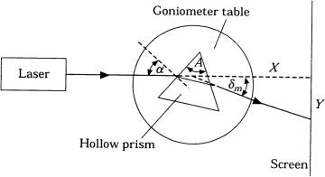
248	Methods and Algorithms for the Measurement of the Optical Parameters of Tissues

Figure 2.13 Schematic of the hollow prism refractometer for the measurement of the index of refraction of blood and other bioliquids.742

diabetic patients.754 It was shown that for intact RBCs at physiological pH 7.3, hyperglycation of hemoglobin leads to a higher refractive index; at maximum it increased from 1.55 at normal to 1.65 for diabetics. The increase, followed-up saturation, and damping of the refractive index of solutions of hemoglobin or whole blood with glucose at an increased concentration of glucose were found using OCT measurements.752,753 The results for the hemoglobin solution at concentration of 140 g/l, which is characteristic for blood at normal physiological conditions, are shown in Fig. 2.14.

According to Eq. (2.31), the initial refractive index of the hemoglobin solution of 140 g/l in water with zero concentration of glucose at 820 nm is expected as nHb140 = 1.355. To evaluate the contribution of glucose at different concentrations to the mean refractive index of the solution supposing noninteracting hemoglobin and glucose molecules, the weighted average of refractive indexes [see Eq. (1.151)] of the glucose solution in water, nglw, and hemoglobin, nHb, should be calculated as

nHb+gl = fglwnglw + (1 − fglw)nHb,

(2.35)

where fglw is the volume fraction of the glucose solution. In experiments, the volume fraction of glucose solution was kept constant at fglw = 0.86, which corresponds to a hemoglobin concentration of 140 g/l (14%). In this equation, the refractive index of dry hemoglobin nHb is presented. The value nglw can be calculated using the expression172,339,340

nglw = nw + 1.515 × 10−6 × Cgl,

(2.36)

where Cgl is the glucose concentration in mg/dl. Since nw can be found for 820 nm from Eq. (1.202) as nw = 1.328 and Cgl is known, nglw can be calculated for each used concentration of glucose.

The refractive index of hemoglobin nHb can be estimated from Eqs. (2.31) and (2.35) when glucose concentration is zero. From Eq. (2.31), it follows that

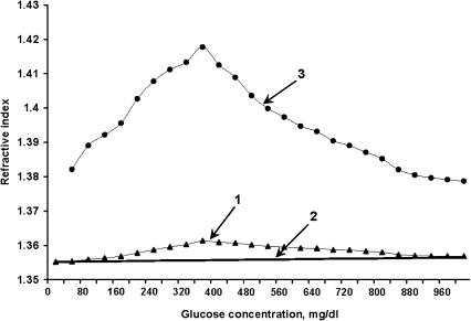
Tissue Optics: Light Scattering Methods and Instruments for Medical Diagnosis

249

Figure 2.14 Experimental and reconstructed data for the refractive index change of human hemoglobin at glucose concentration increase in solution.753 OCT refractometer working on 820 nm, hemoglobin concentration of 140 mg/l at pH = 7.3. (1) Raw data; (2) calculated data using Eqs. (2.35) and (2.36) for noninteracting hemoglobin and glucose; (3) reconstructed on the basis of Eq. (2.37), refractive index of the glycated hemoglobin fraction.

nHb140 = 1.355; thus, from Eq. (2.35), nHb140 = fwnw + (1 − fw)nHb, and for fw = 0.86 and nw = 1.328, nHb = 1.521, which correlates with experimental data for the refractive index of dried RBCs of normal blood.754 Therefore, nHb+gl can be found for solutions with different glucose concentrations and a constant concentration of hemoglobin. As it follows from Eq. (2.35), the mean refractive index for noninteracting molecules at an increase of glucose concentration of 10 times (from 40 to 400 mg/dl) causes only a slight increase of the refractive index in the range from 1.355 to 1.356 [see linear dependence (2) in Fig. 2.14].

In contrast, the experimental data show that the refractive index of a hemoglobin solution at an increase of glucose concentration from 40 to 400 mg/dl changes more effectively, from 1.355 to 1.361 [curve (1) in Fig. 2.14]. The obtained degree of refractive index increase, its saturation, and subsequent fall evidently can be explained using the concept of glucose and hemoglobin molecules interaction when different forms of glycated hemoglobin with new molecular structures and optical properties are originated.756 The volume fraction of glycated hemoglobin (GHb) in the blood of diabetic patients linearly depends on the mean blood glucose (MBG)

in the plasma, which is described by the following empirical equation:756
fGHb = 2.7 × 10−4 MBG(mg/dl) + 0.058.	(2.37)

This relation allows one to reconstruct the refractive index of the glycated portion of the total hemoglobin using the general relationship, Eq. (2.35). The ﬁnal result

250	Methods and Algorithms for the Measurement of the Optical Parameters of Tissues

of the reconstruction is presented by curve (3) in Fig. 2.14. To understand the behavior of the index of refraction of glycated hemoglobin, the classical theory of light dispersion in condensed matter can be used. This theory gives the following formula for the refractive index:757

q2
n = 1 + αN M ,	(2.38)

where α is the wavelength-dependent coefﬁcient, N is the number of molecules, M is the molecule’s mass, and q is the molecule’s charge. From this equation, it follows that the refractive index of hemoglobin depends on molecular weight and charge only: it is a square-law function of charge and an inversely proportional function of molecular weight. Each protein has several different side groups (R), which deﬁne a molecule’s charge. As it follows from Ref. 754, the charge of an R-group of hemoglobin molecules may be increased at glucose binding, but at the same time the increased mass of glycated hemoglobin molecules decreases the refractive index. These facts may explain the obtained changes of refractive index in the experiments. At glucose concentrations from 40 to 200–300 mg/dl, the increase in charge of the R-group of glycated hemoglobin molecules is higher than that of molecular weight and the refractive index increases. At glucose concentrations higher than 200–300 mg/dl due to signiﬁcant increase of M and charge saturation, refractive index dependence saturates and even falls with glucose concentration.

Some other reasons may also affect the refractive index change, such as uncontrolled hemoglobin oxygen saturation (see Fig. 2.13)750,751 and/or increase of

the hemoglobin’s afﬁnity to oxygen at glucose elevation (up to 200% increase in afﬁnity for 15–20 mM of glucose was found by the authors of Ref. 758).

Because the refractive index of tissue and blood components deﬁnes their scattering properties, measured scattering parameters may have an advantage to

evaluate the refractive index of tissue and blood components and their mean values.703,721,759–761 Let us discuss this technique in more detail.759 For a monodis-

perse system of spherical scatterers, the reduced scattering coefﬁcient can be described by the following expression, written in a more general form than Eq. (2.24):

μs = N0πaF (fs)Qs(ns, n0, a, λ)(1 − g),

(2.39)

where N0 is the number of scatterers in a unit volume, a is their radius, F (fs) is the function accounting for the density of particle packing, fs is the volume fraction of scatterers, ns is the refractive index of the scatterers, ns is the refractive index

of the ground material, λ is the wavelength, and Qs and g are factors of scattering efﬁciency and anisotropy, which are calculated from Mie theory.129,146,148

Determination of the reduced scattering coefﬁcient of a tissue sample using integrating sphere or spatially resolved techniques and corresponding algorithms for extraction of the scattering coefﬁcient, such as inverse adding-doubling or Monte Carlo, the knowledge of the refractive indices of the scatterers and the ground material at one of the wavelengths, as well as experimental or theoretical estimations

Tissue Optics: Light Scattering Methods and Instruments for Medical Diagnosis

251

for mean radius of the scatterers, allows one to solve the inverse problem and reconstruct the spectral dependence of the refractive index of the scatteres for a given spectral dependence of the refractive index of the ground material.759 Similar measurements and theoretical estimations done for a tissue sample before and after its prolonged bathing in saline or other biocompatible liquid with known optical characteristics allow one to evaluate the spectral dependencies of the refractive index of the scatterers and the ground material.

Let us consider a few examples. The major scatterers in human sclera are long

collagen ﬁbers with a wide range of diameters and a mean value of 100 nm. Fibers are arranged quasi-randomly in the bundles (see Chapter 3).723,762 Due to the char-

acteristic structure sizing and multiple crossings of bundles, this system can be approximated by a monodisperse system of spherical scatterers with similar spectral properties. In that case, the Mie-equivalent scatterer radius is equal to 250 nm. This value of particle radius is ﬁtted to values of Mie-equivalent radius received for in vivo measurements of skin, in which the scattering properties are mostly deﬁned by the dermis—also ﬁbrous tissue [see Eqs. (1.180) and (1.181)]. Using experimental spectral dependence for the reduced scattering coefﬁcient and accounting for a scleral sample that has been placed into a physiological solution for a long time, the interstitial ﬂuid was therefore replaced by a physiological solution whose refractive index is close to water, the spectral dependence for refractive index of the scatterers was reconstructed.703,760 The spectral dependence for water, described by Eq. (1.202), was used at reconstruction. The following approximated formula for the refractive index of the material of effective scatterers of scleral tissue valid within the spectral range from 400 to 800 nm was received as a ﬁnal result of the reconstruction:

nc(λ) = 1.4389 + 1.5880 × 104λ−2 − 1.4806 × 109λ−4 + 4.3917 × 1013λ−6. (2.40)

In fact, this dispersion relation should be close to the spectral dependence of the index of refraction of hydrated collagen because 75% of sclera’s dry weight is due to collagen.723 The estimated value of the refractive index of normally hydrated scleral collagen (68% of hydration for a whole tissue) of n = 1.474,172 corresponding to direct refraction measurements for whole sclera at a wavelength of 589 nm,723 is well ﬁtted to the value calculated from this semi-empirical relation.

The similar analysis of experimental data of the scattering properties of normal and immersed human skin in the spectral range from 400 to 700 nm allows one to reconstruct spectral dependences of both refractive indices for material of effective scatterers nss(λ) and ground (interstitial liquid) material nsi(λ) as703

nss(λ) = 1.4776 − 1.7488 × 104λ−2 + 6.7270 × 109λ−4 − 3.3390 × 1014λ−6, (2.41)

nsi(λ) = 1.3510 + 2.1342 × 103λ−2 + 5.7893 × 108λ−4 − 8.1548 × 1013λ−6. (2.42)

252	Methods and Algorithms for the Measurement of the Optical Parameters of Tissues

Using the law of Gladstone and Dale [Eq. (1.150)] and these expressions, one can derive the dispersion formula for a whole skin as703

nskin(λ) = 1.3090 − 4.3460 × 102λ−2 + 1.6065 × 109λ−4 − 1.2811 × 1014λ−6. (2.43)

This is a more precise formula for describing the refractive index of skin than Eq. (2.26), which was received from the simplest suppositions for a skin model as a mixture of water and proteins with a constant refractive index.

For tissue optics, this is of great importance to know the dispersion properties of melanin, which is contained in skin, hairs, eye sclera and iris, and other tissues. Melanin granules are the major back-reﬂecting particles in OCT and small-scale spatially resolved spectroscopy of skin. The above-described spectroscopic studies of water suspensions of natural melanin, where the mean radius of particles was determined using electronic microscopy, allow us to solve the inverse problem

and to reconstruct the wavelength dependence of the refractive index of melanin particles in the range from 350 to 800 nm as703,761

nM(λ) = 1.6840 − 1.8723 × 104λ−2 + 1.0964 × 1010λ−4 − 8.6484 × 1014λ−6. (2.44)

An original method for measuring the refractive indices of dentine matrices, based on optical immersion and taking advantage of its tubular structure and the ability to transmit light as in a waveguide, was proposed in Ref. 763. Using this method for freshly cut teeth, n0 was found to be 1.553 ± 0.001 for visible light.

A short-pulse time-delay technique was also successfully applied for refractive index estimation of normal breast tissue (of thickness d = 0.8 mm) and malignant breast tissue (d = 0.85 mm).31 Using the known thickness of the sample and the measured shift t of the transmitted pulse peak relative to the delay time measured through a layer of air of the same thickness, the mean phase refractive index n¯ of a tissue sample can be calculated. Very short pulses should be used in such measurements; thus, a group of different wavelengths propagates in a media and the material dispersion (dn/d¯ λ) should be accounted for by introducing the group refractive index

¯ g = ¯ −			dλ
n	n	λ		dn¯	.	(2.45)

The time delay in the pulse arrival for a tissue sample of thickness d is31

t = (n¯ g1 − ng2), (2.46) c0

where c0 is the light velocity in a vacuum, n¯ g1 is the effective (mean) group refractive index of a tissue, and ng2 is the group refractive index of the homogeneous reference medium (air). The effective group refractive index of a tissue is

n¯ g1 = fsngs + (1 − fs)ng0,

(2.47)

Tissue Optics: Light Scattering Methods and Instruments for Medical Diagnosis

253

where fs is the volume fraction of the scatterers composing a tissue, ngs is the group refractive index of the scatterers, and ng0 is the group refractive index of the ground material of a tissue. The values of the phase refractive index of the abovementioned two samples were calculated to be n¯ = 1.403 for normal and 1.431 for malignant tissue.31

As it was already shown, OCT dynamic and spatially conﬁned measurements

of refractive index and scattering coefﬁcients of tissue and blood are very important for the monitoring of physiological changes in living tissues.737,711–713,716–718,720, 750–753 For basic principles and applications of OCT, see Chapters 4 and 9. OCT

provides simple and straightforward measurements of the index of refraction both in vitro and in vivo.423,712,713,737,750–753,765–777 The in-depth scale of OCT images

is determined by the optical path length zopt between two points along the depth direction. Because a broadband light source is used, the optical path length is proportional to the group refractive index ng and geometrical path length z as693

zopt = ng z.

(2.48)

Usually, ng = n. This simple relation is valid for a homogeneous medium and can be used in in vitro studies when geometrical thickness of a tissue sample z is known.

Sometimes both the refractive index and thickness of a tissue sample should

be measured simultaneously. In that case, a two-step procedure can be applied.765, 767,772 First, a stationary mirror is placed in the sample arm of an interferometer to

get the geometric position of the mirror supposing that the group refractive index of air is 1(z1). Then a tissue sample with unknown index ng and thickness d should be placed before the mirror in the sample arm. Two peaks from the anterior (z2) and the posterior (z3) surfaces of the sample will appear with the distance between them equal to a sample optical thickness [see Eq. (2.48)], and the position of the mirror (z4) will be shifted by (ng − 1)d due to the sample whose group refractive index is greater than that of air. Thus, the calculation of the geometrical thickness and the group refractive index proceeds as follows:

− 2

−

− 1

g =

z )

z ), n

(2.49)

For in vivo measurements of the index of refraction, a focus-tracking method that uses OCT to track the focal-length shift that results from translating the focus of

an objective along the optical axis within a tissue was introduced767 and further developed.712,713,768–771 For the refractive index evaluation, the coincidence of the

maxima of the interference pattern and spatial focus, registered as a signal maximum, is needed. At least two points along the depth direction have to be probed to estimate a mean value of the refractive index between them. Usually a multistep measurement is provided. The geometric average refractive index for a ﬁber/lens

254 Methods and Algorithms for the Measurement of the Optical Parameters of Tissues

focus tracking system is deﬁned by the following expression:712,713
n	√			nobj		,	(2.50)
		ngn

˜ =			=	1 − zFiber
					zL1

where nobj is the refractive index of the objective in the sample arm, zL1 is the change of position of the ﬁrst objective lens, and zFiber is the ﬁber tip position in the sample arm. The difference between both refractive indices is usually small, only a few percent, and can be ignored in practice. For a piecewise homogeneous medium along the depth direction, the slope zL1/ zFiber has to be evaluated at the focus tracked condition ( zL1 positioned for maximum signal).

A bifocal optical coherence refractometer, which is based on the measurements

of the optical path length difference between two foci simultaneously, was recently suggested.770,771 The main advantage of this technique is that it avoids the need to

physically relocate the objective lens or the sample during an axial scan. At employment of a relatively low numerical aperture (NA) objective lens in the sample arm, the ratio of the optical path length difference between two foci, measured in the medium, zf–opt, and in air, zf, is described by the expression771

		1
zf–opt		1	(NA)2	1
zf	≈ ngn 1 +	2	(NA)2	1 − n2	.	(2.51)

For a typical value of tissue index of refraction n = 1.4 and NA = 0.2, the second term in the square parentheses is of only 1% of the magnitude of the ratio.

Accounting for this estimation and that ng = n, a much simple relation, as used in Ref. 712, can be found as

zf–opt ≈ n2 zf.

(2.52)

Received relations [see Eqs. (2.48)–(2.52)] for refractive index evaluation supposed homogeneous media under study. Tissues and blood are inhomogeneous media with a high scattering. Thus, these relations should be modiﬁed. For example, the modiﬁed Eq. (2.48) can be applied for describing dynamic OCT images for blood samples at sedimentation (see Fig. 2.15).737 The OCT image demonstrates that in a process of blood sedimentation, the mean refractive index of a blood layer is reduced (the line, showing the reﬂectance of the posterior surface of a cuvette, is moving up with time). Such behavior can be understood through the mechanism of the reduction of the bulk scattering due to cell aggregation.

When the refractive index of the scatters ns differs little from the ground medium n0, the scattered ﬁeld Esc(r ) at position r can be written as the following

iterative series:402
Esc(r ) = αE1(r ) + α2E2(r ) + · · · ,	(2.53)

Tissue Optics: Light Scattering Methods and Instruments for Medical Diagnosis	255
where
α = (ns − n0)/2πn0.	(2.54)

The ﬁrst term in Eq. (2.53) accounts for single-scattering events, the RayleighGans approximation; the second term accounts for all double-scattering events. Values of Esc(r ) in the direction of propagation of the incident light (along the positive z-axis) make up the “forward-scattered light.” This portion of the scattered light adds to the incident wave, slightly changing both its phase and magnitude, which can be expressed as402

exp ik z + L n0		,	(2.55)
	n

where k = 2π/λ is the wave number, λ is the wavelength within the medium of index n0, and L is the thickness of the scattering medium. The real part of the quantity n gives a phase change of the transmitted light, so it should be interpreted as an index change of the medium due to light scattering. The imaginary part of n leads to an exponential decay of the transmitted wave caused by the scattered light escaping from the propagating light.

The refractive index n of the medium is402


n	=	n	0	+	n	n	n2 − n¯ 2		Q(λ/ l	),	(2.56)
n		n			n	n			Q(λ/ l	),	(2.56)
						= ¯ +		n	c
							¯

where n¯ is deﬁned by the refractive indices of tissue or blood compounds [see Eq. (1.150)]; for a two-compound medium it is equal to

n¯ = fsns + (1 − fs)n0,

(2.57)

where fs is the volume fraction of scattering particles; n2 is the mean-square value of refractive index ﬂuctuations, Q(λ/ lc) refers to the form of scatters and their aggregation, and lc is the correlation length of randomly distributed refractive index ﬂuctuations. Q = 1.17 in the limit of large correlation length, lc λ (large particles), and Q = 0 in the limit of small lc (Rayleigh limit). In the case that index ﬂuctuations take the form of parallel cylinders, Q = 0.67 for the large lc.

In the process of blood sedimentation, the two-phase system of plasma and RBCs is formed. Each phase has its own volume (thickness after separation) and refractive index. Let us deﬁne the time-dependent thickness of the RBC layer as H (t), then the thickness of the upper clear plasma is [L − H (t)] (see Fig. 2.15). The averaged refractive index of the layer of thickness L, containing two layers with different refractive indices, can be written in the form

n		(t)	=	[L − H (t)]	n	H (t)	n	,	(2.58)

	sed			L	¯ +	L

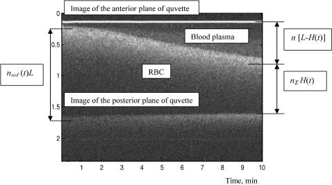
256	Methods and Algorithms for the Measurement of the Optical Parameters of Tissues

Figure 2.15 Blood sedimentation in a cuvette of L = 1.1 mm in thickness. Dynamic OCT in-depth image (λ = 820 nm) of whole blood sample slightly diluted by saline (13%) taken from a healthy volunteer (woman, 35 years old).737

where n and n¯ are deﬁned by Eqs. (2.56) and (2.57). Because of n always being larger than n¯ and the sedimentation process in general is expressed as H (t)/L → Hct (blood hematocrit), then the total refractive index must go down with time.

For describing the inﬂuence of time-dependent refractive index changes on OCT images during blood sedimentation, n should be replaced by n in Eq. (2.48). The initial refractive index before sedimentation is started can be estimated from experimental the OCT image presented in Fig. 2.15 for whole blood slightly diluted by saline. The experimental value of zopt (distance between upper and lower bright lines at zero time) is equal to 1.533 mm or for thickness of the blood

vessel z	=	=	=	1.394. Ac-
vessel z		1.1 mm, from relation zopt n z we can ﬁnd n		1.394. Ac-

counting for the fact that the whole blood refractive index is nb = 1.400, we can estimate the expected value of the refractive index n (t = 0) from n (t = 0) = fbnb + (1 − fb)nsaline, where fb is the volume fraction of whole blood in the sample and nsaline is the index of saline. For fb = 0.87 and nsaline = 1.330, the expected value of n = 1.391 is well ﬁtted to the measured one.

The experimental value of zopt at 10 min is equal to 1.483 mm; thus, nsed(t = 10 min) = 1.348. Accounting for this, from the OCT image, where

(L − H )/L = 0.55, H /L = 0.45, and n¯ = fbpnbp + (1 − fbp)nsaline = 0.87 × 1.340 + 0.13 × 1.33 = 1.339, we can evaluate n from Eq. (2.58) as n = 1.359 and the corresponding relative index ﬂuctuations of the RBC layer from Eq. (2.56)


as [(n2	− ¯ ¯ ] =		=
as [(n2	n2)/n	0.017 for Q		1.17.

Results of in vitro and in vivo measurements of phase and group refractive indices of tissue, blood, and their compounds using the technique discussed and some other techniques are summarized in Table 2.6.

<<< < Предыдущая 1 2 3 4 56 / 146 7 8 9 10 11 12 13 14 > Следующая >>>

Соседние файлы в предмете [НЕСОРТИРОВАННОЕ]

#
21.03.2016255.5 Кб4Psikhologia_obschenia_Lektsia3.pdf
#
21.03.2016374 Кб4Psikhologia_obschenia_Lektsia4.pdf
#
28.04.2019114.18 Кб1Pupils`cards .doc
#
20.03.2016131.07 Кб6QuestionsMin3semestr2013.doc
#
20.03.2016493.06 Кб5Rabochaya_programma_Pravovedenie_080200.doc
#
21.03.201638.9 Mб17Rasseyanie_Tuchin.pdf
#
26.09.2019601.58 Кб7RAZDEL_9.docx
#
20.03.201635.14 Кб6Razval_nauki_i_obrazovania.docx
#
14.04.2015997.9 Кб53RCv2.pdf
#
09.11.2019227.33 Кб4RD_AS.doc
#
20.09.20193.99 Mб10referat-1.doc