


Preface to the Second Edition
This is the second edition of the tutorial Tissue Optics: Light Scattering Methods and Instruments for Medical Diagnosis first published in 2000. The last seven years, since the printing of the first edition, have seen intensive growth of re-
search and development in tissue optics, particularly in the field of tissue diagnostics and imaging.103–147 Further developments of light-scattering techniques
for the quantitative evaluation of optical properties of normal and pathological tissues and cell ensembles have occurred. New results on theoretical and experimental investigations into light transport in tissues and methods for solving direct and inverse scattering problems for random media with multiple scattering
and quasi-ordered media have been found. A few specific fields, such as optical coherence tomography (OCT)108–111,115,116,126,127,129,130,136,142 and polarizationsensitive technologies,129,130,135,136,138,139 which are very promising for optical
medical diagnostics and imaging, have developed rapidly over the last few years. The optical clearing method, based on reversible reduction of tissue scattering due
to refractive index matching of scatterers and ground matter, has also been of great interest for research and application since the last edition.129,132,136,139,140 Further developments of Raman and vibrational spectroscopies104,105,123,130,132,136,143 and multiphoton microscopy114,119,122,130,132,136,137 applied to morphology and the
functioning of living cells and tissues have been provided by many research groups. This new edition of this book is conceptually the same as the first one. It is also divided into two parts: Part I describes tissue optics fundamentals and basic research, and Part II presents optical and laser instrumentation and medical applications. The author has corrected misprints, updated the references, and added some new results mostly on tissue optical properties measurements (Chapter 2) and polarized light interaction with turbid tissues (Section 1.4). Recent results on polarization imaging and spectroscopy techniques (Chapter 7), as well as on OCT developments and applications (Chapter 9) are also overviewed. Materials on controlling tissue optical properties (Chapter 5) and optothermal and optoacoustic interactions of light with tissues (Section 1.5) are updated. Brief descriptions of fluorescent,
nonlinear, and inelastic light scattering spectroscopies are provided in Chapter 1. I am grateful to Sharon Streams for her suggestion to prepare the second edition
of the tutorial and for her assistance in editing of the book. I also would like to thank Merry Schnell for her assistance on the final stage of book editing and production.
I am very thankful to attendees of my short courses “Coherence, Light Scattering, and Polarization Methods and Instruments for Medical Diagnosis,” “Tissue Optics and Spectroscopy,” “Tissue Optics and Controlling of Tissue Optical Properties,” and “Optical Clearing of Tissues and Blood,” which I have given during
xxxix
xl |
Preface to the Second Edition |
SPIE Photonics West Symposia, SPIE/OSA European Conferences on Biomedical Optics, and OSA CLEO/QELS Conferences over last seven years, for their stimulating questions, fruitful discussions, and critical evaluations of presented materials. Their responses were very valuable for preparation of this edition. My joint chairing with Joseph A. Izatt and James G. Fujimoto of the SPIE Conference on Coherence Domain Optical Methods and Optical Coherence Tomography in Biomedicine also was very helpful.
The original part of this work was supported within the Russian and international research programs by grant N25.2003.2 of President of Russian Federation “Supporting of Scientific Schools,” grant N2.11.03 “Leading ResearchEducational Teams,” contract No. 40.018.1.1.1314 “Biophotonics” of the Ministry of Industry, Science and Technologies of RF, grant REC-006 of CRDF (U.S. Civilian Research and Development Foundation for the Independent States of the Former Soviet Union) and the Russian Ministry of Education, the Royal Society grants for a joint projects between Cranfield University (UK) and Saratov State University, grants of National Natural Science Foundation of China (NSFC), grant of Federal Agency of Education of RF No. 1.4.06, RNP.2.1.1.4473, CRDF grants BRHE RUXO-006-SR-06 and RUB1-570-SA-04, and by Palomar Medical Technologies Inc., MA, USA.
I greatly appreciate the cooperation, contributions, and support of all my colleagues from Optics and Biomedical Physics Division of Physics Department and Research-Educational Institute of Optics and Biophotonics of Saratov State University, especially A. N. Bashkatov, I. V. Fedosov, E. I. Galanzha, E. A. Genina,
I.L. Maksimova, I. V. Meglinski, V. I. Kochubey, V. P. Ryabukho, A. B. Pravdin,
G.V. Simonenko, Yu. P. Sinichkin, S. S. Ul’yanov, D. A. Yakovlev, and D. A. Zimnyakov.
I would like to thank all my numerous colleagues and friends all over the world for collaboration and sending materials which were used in this tutorial and made my work much easier, especially P. E. Andersen, J. F. de Boer, Z. Chen,
P.M. W. French, J. G. Fujimoto, V. M. Gelikonov, P. Gupta, C. K. Hitzenberger,
J.A. Izatt, S. L. Jacques, A. Kishen, S. J. Kirkpatrick, A. Knüttel, J. R. Lakowicz, K. V. Larin, G. W. Lucassen, Q. Luo, B. R. Masters, K. Meek, G. Mueller,
F.F. M. de Mul, L. T. Perelman, A. Podoleanu, A. V. Priezzhev, F. Reil, J. Rodriguez, H. Schneckenburger, A. M. Sergeev, A. N. Serov, N. M. Shakhova,
B.J. Tromberg, L. V. Wang, R. K. Wang, A. J. Welch, A. N. Yaroslavskaya,
I.V. Yaroslavsky, P. Zhakharov, and V. P. Zharov, R. Myllylä, S. A. Boppart,
M.Meinke, A. Mahadevan-Jansen, T. Troy, L. Oliveira, M. Pais Clemente, and
X.H. Hu.
I express my gratitude to my wife, Natalia, and all my family, especially to my daughter, Nastya, and grandchildren, Dasha, Zhenya, and Stepa, for their indispensable support, understanding, and patience during my writing this book.
Valery Tuchin
June 2007

1
Optical Properties of Tissues with Strong (Multiple) Scattering
This first chapter introduces the problem of light (laser beams) transport within strongly (multiple) scattering tissues such as skin, breast, brain, and vessel walls. Basic principles and theoretical descriptions using radiation transfer theory or Monte Carlo (MC) simulation are considered. The propagation of short pulses and photon-density diffusion waves in scattering and absorbing media is analyzed, and the prospects of these methods for tissue spectroscopy and tomography are discussed. Tissue structure and anisotropy, polarization phenomena, optothermal, optoacoustic, and acoustooptical interactions in strongly scattering tissues are described. A discrete-particle model of soft tissue is presented. Fluorescence and inelastic light scattering, including multiphoton fluorescence and vibrational and Raman spectroscopies, are discussed. The design and characterization of tissuelike phantoms for optical diagnostics and light dosimetry are described.
1.1 Propagation of continuous-wave light in tissues
1.1.1 Basic principles, and major scatterers and absorbers
Biological tissues are optically inhomogeneous and absorbing media whose average refractive index is higher than that of air. This is responsible for partial reflection of the radiation at the tissue/air interface (Fresnel reflection), while the remaining part penetrates the tissue. Multiple scattering and absorption are responsible for laser beam broadening and eventual decay as it travels through a tissue, whereas bulk scattering is a major cause of the dispersion of a large fraction of radiation in the backward direction. Therefore, light propagation within a tissue depends on the
scattering and absorption properties of its components: cells, cell organelles, and various fiber structures.1–3,15,129,130,134,138 The size, shape, and density of these
structures; their refractive index relative to the tissue ground substance; and the
polarization states of the incident light all play important roles in the propagation
of light in tissues.1–3,15,129,130,134,138,145–153
In view of the great diversity and structural complexity of tissues, the development of adequate optical models that account for the scatter and absorption of light is often the most complex step of a study. Two approaches are currently used for tis-
sue modeling. In the framework of the first one, tissue is modeled as a medium with a continuous random spatial distribution of optical parameters;3,129,154,155 the second one considers tissue as a discrete ensemble of scatterers.1–3,15,129,130,134,138,156
3
4 |
Optical Properties of Tissues with Strong (Multiple) Scattering |
The choice of the approach is dictated by both the structural specificity of the tissue under study and the kind of light scattering characteristics that are to be obtained.
Most tissues are composed of structures with a wide range of sizes, and most
can be described as a random continuum of inhomogeneities of the refractive index with a varying spatial scale.154,155 Phase contrast microscopy has been used
in particular to show that the structure of the refraction index inhomogeneities in mammalian tissues is similar to the structure of frozen turbulence in a number of cases.154 This fact is of fundamental importance for understanding the peculiarities of light propagation in tissue, and it may be a key to the solution of the inverse problem of tissue structure reconstruction. This approach is applicable for tissues with no pronounced boundaries between elements that feature significant
heterogeneity. The process of scattering in these structures may be described under certain conditions using the model of a phase screen.75,136,155,157
The second approach to tissue modeling is its representation as a system of discrete scattering particles. In particular, this model has been advantageously used
to describe the angular dependence of the polarization characteristics of scattered radiation.145,146,148,150,158 Blood is the most important biological example of a disperse system that entirely corresponds to the model of discrete particles.48,101,159
Biological media are often modeled as ensembles of homogeneous spherical particles, since many cells and microorganisms, particularly blood cells, are close in shape to spheres or ellipsoids. A system of noninteracting spherical particles is
the simplest tissue model. Mie theory rigorously describes the diffraction of light in a spherical particle.148,160 The development of this model involves taking into
account the structures of the spherical particles, namely, the multilayered spheres and the spheres with radial nonhomogeneity, anisotropy, and optical activity.145,146
Because connective tissue consists of fiber structures, a system of long cylinders is the most appropriate model for it. Muscular tissue, skin dermis, dura mater, eye cornea, and sclera belong to this type of tissue formed essentially by collagen fibrils. The solution of the problem of light diffraction in a single homogeneous or multilayered cylinder is also well understood.148
The sizes of cells and tissue structure elements vary in size from a few tenths
of nanometers to hundreds of micrometers.47,58,94–96,129,130,135,138,149–153,161–180
Blood cells (erythrocytes, leukocytes, and platelets) exhibit the following parameters. A normal erythrocyte in plasma has the shape of a concave-concave disk with a diameter varying from 7.1 to 9.2 μm, a thickness of 0.9–1.2 μm in the center and 1.7–2.4 μm on the periphery, and a volume of 90 μm3. Leukocytes are formed like spheres with a diameter of 8–22 μm. Platelets in the bloodstream are biconvex disklike particles with diameters ranging from 2 to 4 μm. Normally, blood has about 10 times as many erythrocytes as platelets and about 30 times as many platelets as leukocytes.
Most other mammalian cells have diameters in the range of 5–75 μm. In the epidermal layer, the cells are large (with an average cross-sectional area of about 80 μm2) and quite uniform in size. Fat cells, each containing a single lipid droplet that nearly fills the entire cell and therefore results in eccentric placement of the
Tissue Optics: Light Scattering Methods and Instruments for Medical Diagnosis |
5 |
cytoplasm and nucleus, have a wide range of diameters, from a few microns to 50–75 μm. Fat cells may reach diameters of 100–200 μm in pathological cases.
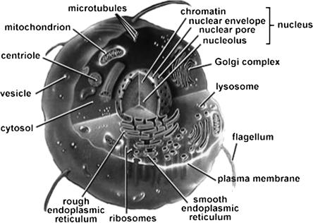
There are a wide variety of structures within cells that determine tissue light scattering (see Fig. 1.1). Cell nuclei are on the order of 5–10 μm in diameter; mitochondria, lysosomes, and peroxisomes have dimensions of 1–2 μm; ribosomes are on the order of 20 nm in diameter; and structures within various organelles can have dimensions of up to a few hundred nanometers. Usually, the scatterers in cells are not spherical. The models of prolate ellipsoids with a ratio of the ellipsoid axes between 2 and 10 are more typical.
Figure 1.1 Major organelles and inclusions of the cell.129
The hollow organs of the body are lined with a thin, highly cellular surface layer of epithelial tissue, which is supported by underlying, relatively acellular connective tissue. In healthy tissues, the epithelium often consists of a single wellorganized layer of cells with en face diameter of 10–20 μm and height of 25 μm (see Fig. 1.2). In dysplastic epithelium, cells proliferate and their nuclei enlarge and appear darker (hyperchromatic) when stained.150 Enlarged nuclei are primary indicators of cancer, dysplasia, and cell regeneration in most human tissues.
In fibrous tissues or tissues containing fiber layers (cornea, sclera, dura mater, muscle, myocardium, tendon, cartilage, vessel wall, retinal nerve fiber layer, etc.) and composed mostly of microfibrils and/or microtubules, typical diameters of the cylindrical structural elements are 10–400 nm. Their length is in a range from 10– 25 μm to a few millimeters.

6 |
Optical Properties of Tissues with Strong (Multiple) Scattering |
Figure 1.2 Microphotograph of the isolated normal intestinal epithelial cells (a) and intestinal malignant cell line T84 (b). Note the uniform nuclear size distribution of the normal epithelial cell (a) in contrast to the T84 malignant cell line, which at the same magnification shows larger nuclei and more variation in nuclear size (b). Solid bars equal 20 μm in each panel (from Ref. 150 © 1999 IEEE).
The dominant scatterers in an artery may be the fibers, cells, or subcellular organelles. Muscular arteries have three main layers. The inner intimal layer consists of endothelial cells with a mean diameter of less than 10 μm. The medial layer consists mostly of closely packed smooth muscle cells with a mean diameter of 15–20 μm; small amounts of connective tissue, including elastin, collagenous, and reticular fibers, as well as a few fibroblasts, are also located in the medial. The outer adventitial layer consists of dense fibrous connective tissue that is largely made up of 1- to 12-μm-diameter collagen fibers and thinner, 2- to 3-μm-diameter elastin fibers.
Another two examples of complex scattering structures are the myocardium and the retinal nerve fiber layer. The myocardium consists mostly of cardiac muscle, which is comprised of myofibrils (about 1 μm in diameter) that in turn consist of cylindrical myofilaments (6–15 nm in diameter) and aspherical mitochondria (1–2 μm in diameter). The retinal nerve fiber layer comprises bundles of unmyelinated axons that run across the surface of the retina. The cylindrical organelles of the retinal nerve fiber layer are axonal membranes, microtubules, neurofilaments, and mitochondria. Axonal membranes, like all cell membranes, are thin (6–10 nm) phospholipid bilayers that form cylindrical shells enclosing the axonal cytoplasm. Axonal microtubules are long tubular polymers of the protein tubulin with an outer diameter of ≈25 nm, an inner diameter ≈15 nm, and a length of 10–25 μm. Neurofilaments are stable protein polymers with a diameter ≈10 nm. Mitochondria are ellipsoidal organelles that contain densely involved membranes of lipid and protein. They are 0.1–0.2 μm thick and 1–2 μm long.
For some tissues, the size distribution of the scattering particles may be essentially monodispersive, and for others it may be quite broad. Two opposing
Tissue Optics: Light Scattering Methods and Instruments for Medical Diagnosis |
7 |
examples are a transparent eye cornea stroma, which has a sharply monodisper-
sive distribution, and a turbid eye sclera, which has a rather broad distribution of collagen fiber diameters.129,130 There is no universal distribution size func-
tion that would describe all tissues with equal adequacy. In optics of dispersed systems, Gaussian, gamma, or power size distributions are typical.171 Polydispersion for randomly distributed scatterers can be accounted for by using the gamma-
distribution or the skewed logarithmic distribution of scatterers’ diameters, cross sections, or volumes.61,129,154,156,165,172 In particular, for turbid tissues such as eye
sclera, the gamma radii distribution function is applicable.61,172
Absorbed light is converted to heat or radiated in the form of fluorescence; it is also consumed in photobiochemical reactions. The absorption spectrum depends on the type of predominant absorption centers and water content of tissues
(see Figs. 1.3–1.7). Absolute values of absorption coefficients for typical tissues
lie in the range 10−2 to 104 cm−1.1–4,6,9–15,28,29,31,37–42,56,57,72,86–91 In the ultravio-
let (UV) and infrared (IR) (λ ≥ 2000 nm) spectral regions, light is readily absorbed, which accounts for the small contribution of scattering and the inability of radiation to penetrate deep into tissues (only through one or two cell layers). Short-wave visible light penetrates typical tissues as deep as 0.5–2.5 mm, whereupon it undergoes an e-fold decrease of intensity. In this case, both scattering and absorption occur, with 15–40% of the incident radiation being reflected. In the 600–1600-nm wavelength range, scattering prevails over absorption, and light penetrates to a depth of 8–10 mm. Simultaneously, the intensity of the reflected radiation increases to 35–70% of the total incident light (due to backscattering).
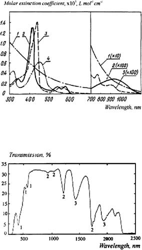
Figure 1.3 The absorption spectrum of water.56
Light interaction with a multilayer and multicomponent skin is a very complicated process.57 The horny-skin layer (stratum corneum) reflects about 5–7% of the incident light. A collimated light beam is transformed to a diffuse one by microscopic inhomogeneities at the air/horny-layer interface. A major part of reflected light results from backscattering in different skin layers (stratum corneum,
8 |
Optical Properties of Tissues with Strong (Multiple) Scattering |
Figure 1.4 Molar attenuation spectra for solutions of major visible light-absorbing human skin pigments: 1, DOPA-melanin (H2O); 2, oxyhemoglobin (H2O); 3, hemoglobin (H2O); 4, bilirubin (CHCl3).57
Figure 1.5 The transmittance spectrum of a 3-mm-thick slab of female breast tissue. A spectrometer with an integrating sphere was used. The contributions of absorption bands of the tissue components are marked: 1, hemoglobin; 2, fat; and 3, water.50
epidermis, dermis, blood, and fat). The absorption of diffuse light by skin pigments is a measure of bilirubin content, hemoglobin concentration, and its saturation with oxygen, and the concentration of pharmaceutical products in blood and tissues; these characteristics are widely used in the diagnosis of various diseases (see Fig. 1.4). Certain phototherapeutic and diagnostic modalities take advantage of ready transdermal penetration of visible and near-infrared (NIR) light inside the body in the wavelength region, corresponding to the therapeutic or diagnostic window (600–1600 nm) (Fig. 1.7).
Another example of heterogeneous multicomponent tissue is a female breast (which is principally composed of adipose and fibrous tissues). The absorption bands of hemoglobin, fat, and water are clearly seen in vitro in the measured spec-
Tissue Optics: Light Scattering Methods and Instruments for Medical Diagnosis |
9 |
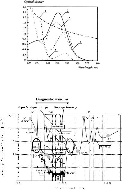
Figure 1.6 UV absorption spectra of major chromophores of human skin: 1, DOPA-melanin, 1.5 mg % in H2O; 2, urocanic acid, 104 M in H2O; 3, DNA, calf thymus, 10 mg % in H2O (pH = 4.5); 4, tryptophane, 2 × 10⁴ M (pH = 7); 5, tyrosine, 2 × 10⁴ M (pH = 7).57
Figure 1.7 Absorption spectra of skin and aorta; spectra of tissue components—water (75%), epidermis, melanosome, and whole blood are also presented; diagnostic lasers and their wavelengths as well as diagnostic/therapeutic window and wavelength ranges suitable for superficial and deep spectroscopy are shown (adapted from Ref. 36).
trum of a 3-mm slab of breast tissue presented in Fig. 1.5.50 Measurement was done using the integrating sphere spectrometer. There is a wide window between
10 |
Optical Properties of Tissues with Strong (Multiple) Scattering |
700 and 1100 nm, and narrow ones at about 1300 and 1600 nm, where the lowest percentage of light is attenuated.
Solid tissues such as ribs and the skull, as well as whole blood, are also easily penetrable by visible and NIR light.1–4,6,9–16,36,91,129,130 The relatively good
transparency of skin for long-wave UV light (UVA) depends on DNA, tryptophane, tyrosine, urocanic acid, and melanin absorption spectra and underlies se-
lected methods of photochemotherapy of skin tissues using UVA irradiation (see
Fig. 1.4).3,6,10,57,86,129,130
A collimated (laser) beam is attenuated in a thin tissue layer of thickness d in accordance with the Bouguer-Beer-Lambert exponential law as37
I (d) = (1 − RF)I0 exp(−μtd), |
(1.1) |
where I (d) is the intensity of transmitted light measured using a distant photodetector with a small aperture (on-line or collimated transmittance), W/cm2; RF is the coefficient of Fresnel reflection; at the normal beam incidence, RF = [(n − 1)/(n + 1)]2; n is the relative mean refractive index of tissue and surrounding media; I0 is the incident light intensity, W/cm2;
μt = μa + μs |
(1.2) |
is the extinction coefficient (interaction or total attenuation coefficient), 1/cm, where μa is the absorption coefficient, 1/cm, and μs is the scattering coefficient, 1/cm. Strictly speaking, Eq. (1.1) is valid only for a highly absorbing media, when μa μs.
The extinction coefficient is connected with the extinction cross section σext as
μt = ρsσext, |
(1.3) |
where ρs is the density of particles (tissue and cell compounds). For a system of particles with absorption,
σext = σsca + σabs, |
(1.4) |
and |
|
μs = ρsσsca, μa = ρsσabs. |
(1.5) |
The average scattering cross section per particle can be presented in a form suitable for experimental evaluations:148
|
λ2 |
1 |
|
π |
|
|
σsca = |
|
|
|
0 |
I (θ) sin θdθ, |
(1.6) |
2π |
I0 |
|||||
where I0 is the intensity of the incident light, I (θ) is the angular distribution of the scattered light by a particle, and θ is the scattering angle. For macroscopically
Tissue Optics: Light Scattering Methods and Instruments for Medical Diagnosis |
11 |
isotropic and symmetric media, the average scattering cross section is independent of the direction and polarization of the incident light. The average extinction, σext, and absorption, σabs, cross sections are also independent of the direction and polarization state of the incident light.
The probability that a photon incident on a small volume element will survive is equal to the ratio of the scattering and extinction cross sections, and is called the “albedo” for single scattering, :
= |
σsca |
= |
μs |
(1.7) |
|
|
|
. |
|||
σext |
μt |
||||
The albedo ranges from zero for a completely absorbing medium to unity for a completely scattering medium.
The mean free path length (MFP) between two interactions is denoted by
lph = μt−1. |
(1.8) |
1.1.2 Theoretical description
To analyze light propagation under multiple scattering conditions, it is assumed that absorbing and scattering centers are uniformly distributed across the tissue. UV-A, visible, or NIR radiation is normally subject to anisotropic scattering characterized by a clearly apparent direction of photons undergoing single scattering,
which may be due to the presence of large cellular organelles [mitochondria, lysosomes, and inner membranes (Golgi apparatus)].3,58,85,95,96,129,130,135,150–153
When the scattering medium is illuminated by unpolarized light and/or only the intensity of multiply scattered light needs to be computed, a sufficiently strict mathematical description of continuous wave (CW) light propagation in a medium
is possible in the framework of the scalar stationary radiation transfer theory
(RTT).1,3,6,12–16,129,130,135,136,145,146,181–197
This theory is valid for an ensemble of scatterers located far from one another and has been successfully used to work out some practical aspects of tissue optics. The main stationary equation of RTT for monochromatic light has the form1
∂s ¯ |
= − |
t |
¯ ¯ + |
4π 4π |
¯ ¯ |
¯ ¯ |
|
|
|
∂I (r¯, s) |
|
μ |
I (r, s) |
μs |
I (r, s )p(s, s |
)d |
, |
(1.9) |
|
|
|
|
|||||||
where I (r¯, s)¯ is the radiance (or specific intensity)—average power flux density at point r¯ in the given direction s¯, W/cm2 sr; p(s,¯ s¯ ) is the scattering phase function, 1/sr; and d is the unit solid angle about the direction s¯ , sr. It is assumed that there are no radiation sources inside the medium.
The scalar approximation of the radiative transfer equation (RTE) gives poor accuracy when the size of the scattering particles is much smaller than the wave-
length, but provides acceptable results for particles comparable to and larger than the wavelength.146,184 There is ample literature on the analytical and numerical solutions of the scalar radiative transfer equation.1,3,15,129,130,184–197
12 |
Optical Properties of Tissues with Strong (Multiple) Scattering |
If radiative transport is examined in a domain G R3, and ∂G is the domain boundary surface, then the boundary conditions for ∂G can be written in the following general form:
|
|
|
|
¯ ¯ |
¯ ¯ |
0 = ¯ ¯ + |
ˆ |
¯ ¯ |
¯ ¯ |
0 |
|
(1.10) |
¯ |
|
¯ |
I (r, s) |
(sN )< |
S(r, s) |
RI (r, s) |
(sN )> |
|
, |
|||
|
is the outside |
|
|
|
¯ ¯ |
|
|
|
||||
where r |
∂G, N |
normal vector to ∂G, S(r, s) is the incident light |
||||||||||
distribution at |
∂ |
G, and ˆ |
is the reflection operator. When both absorption and |
|||||||||
|
|
|
R |
|
|
|
|
|
|
|
|
|
reflection surfaces are present in the domain G, conditions analogous to Eq. (1.10) must be given at each surface.
For practical purposes, integrals of the function I (r,¯ s)¯ over certain phase space regions (r,¯ s)¯ are of greater value than the function itself. Specifically, optical probes of tissues frequently measure the outgoing light distribution function at the medium surface, which is characterized by the radiant flux density or irradiance (W/cm2):
|
|
¯ ¯ |
0 |
¯ ¯ |
|
¯ = |
|
¯ |
(1.11) |
||
F (r) |
|
|
I (r, |
s)(sN |
|
|
|
¯ )d , |
|
||
(sN )>
where r¯ ∂G.
In problems of optical radiation dosimetry in tissues, the measured quantity is actually the total radiant-energy-fluence rate U (r)¯ . It is the sum of the radiance over all angles at a point r¯ and is measured by watts per square centimeter:
U (r¯) = I (r,¯ s)¯ d . (1.12)
4π
The phase function p(s,¯ s¯ ) describes the scattering properties of the medium and is in fact the probability density function for scattering in the direction s¯ of a photon traveling in the direction s¯; in other words, it characterizes an elementary scattering act. If scattering is symmetric relative to the direction of the incident wave, then the phase function depends only on the scattering angle θ (angle between directions s¯ and s¯ ), i.e.,
¯ ¯ |
) |
= |
p(θ). |
(1.13) |
p(s, s |
|
The assumption of random distribution of scatterers in a medium (i.e., the absence of spatial correlation in the tissue structure) leads to normalization:
π
p(θ)2π sin θdθ = 1. |
(1.14) |
0
In practice, the phase function is usually well approximated with the aid of the postulated Henyey-Greenstein function:1,3,12–16,70,129,130,164
p(θ) |
= |
1 |
|
1 − g2 |
, |
(1.15) |
|
4π (1 + g2 − 2g cos θ)3/2 |
|||||||
|
|
|
|||||
Tissue Optics: Light Scattering Methods and Instruments for Medical Diagnosis |
13 |
where g is the scattering anisotropy parameter (mean cosine of the scattering angle θ):
π
g ≡ cos θ = p(θ) cos θ · 2π sin θdθ. (1.16)
0
The value of g varies in the range from −1 to 1:145,146 g = 0 corresponds to isotropic (Rayleigh) scattering, g = 1 to total forward scattering (Mie scattering at large particles), and g = −1 to total backward scattering.
The integrodifferential Eq. (1.9) is too complicated to be employed for the analysis of light propagation in scattering media. Therefore, it is frequently simplified by representing the solution in the form of spherical harmonics. Such simplification leads to a system of (N + 1)2 connected differential partial derivative equations known as the PN approximation. This system is reducible to a single dif-
ferential equation of order (N + 1). For example, four connected differential equations reducible to a single diffusion-type equation are necessary for N = 1.191–197
It has the following form for an isotropic medium:
( 2 − μeff2 )U (r¯) = −Q(r),¯ |
(1.17) |
|
where |
|
|
μeff = [3μa(μs + μa)]1/2 |
(1.18) |
|
is the effective attenuation coefficient or inverse diffusion length, |
μeff = 1/ ld, |
|
1/cm; |
|
|
¯ = |
¯ |
(1.19) |
Q(r) |
(cD)−1q(r), |
|
where q(r)¯ is the source function (i.e., the number of photons injected into the unit volume), and
D = |
|
1 |
|
(1.20) |
3(μ |
+ |
μa) |
||
|
s |
|
|
|
is the photon diffusion coefficient, cm2/c; |
|
|
|
|
μs = (1 − g)μs |
(1.21) |
|||
is the reduced (transport) scattering coefficient, 1/cm, and c is the velocity of light in the medium. The transport mean free path of a photon (cm) is defined as
|
|
|
|
|
lt = (1/μt) = (μa + μs)−1, |
(1.22) |
where μ |
= |
μa |
+ |
μ |
is the transport coefficient. |
|
t |
|
s |
|
|
14 |
Optical Properties of Tissues with Strong (Multiple) Scattering |
It is worthwhile to note that the transport mean free path (MFP) in a medium with anisotropic single scattering significantly exceeds the MFP in a medium with isotropic single scattering, lt lph [see Eq. (1.8)]. The transport MFP lt is the distance over which the photon loses its initial direction.
Diffusion theory provides a good approximation in the case of a small scat-
tering anisotropy factor g ≤ 0.1 and large albedo → 1. For many tissues, g ≈ 0.6–0.9, and can be as large as 0.990–0.999, for example, for blood.48,49,87,129
This significantly restricts the applicability of the diffusion approximation. It is argued that this approximation can be used at g < 0.9, when the optical thickness τ of an object is of the order 10–20:
d
τ = μtds, (1.23)
0
where d is the tissue depth (thickness) in the direction s.
However, the diffusion approximation is inapplicable for beam input near the object’s surface where single or low-step scattering prevails. When a narrow light beam is normally incident upon a semi-infinite turbid medium with anisotropic scattering, it can be considered as converted into an isotropic point source at the depth of one transport MFP lt [Eq. (1.22)] below the surface. The strength of this point source is the original source strength multiplied by the transport albedo193
|
|
|
μ |
|
|
|
|
= |
|
|
s |
|
|
. |
(1.24) |
μ |
a |
+ |
μ |
|
|||
|
|
|
|
s |
|
|
It was confirmed that diffusion theory is accurate for describing photon migration in infinite, homogeneous, turbid media.34,46,51,93,191,198–206 However, another
procedure of diffusion equation derivation, described in Refs. 34, 51, and 191, in spite of leading to the basic Eq. (1.20) gives a more general expression for the photon diffusion coefficient:
D = |
|
1 |
|
|
, |
(1.25) |
3(μ |
aμ |
) |
||||
|
s |
+ ¯ |
a |
|
|
|
where a¯ is the numerical coefficient depending on the form of the diffusion equa-
tion (on the scattering anisotropy factor).
Systematic approximation schemes lead to recommendations34,51,191 of a¯ = 0, 1/5, 1/3, 1. Any of these a¯ values gives significantly better agreement with random-walk simulations than the diffusion equation at a¯ = 0, with a¯ = 1/3 being slightly better than the two others.191 Because values a¯ = 1/5 and a¯ = 1 lead to the wrong pulse-front propagation speeds, and only the intermediate value a¯ = 1/3
gives the correct speed, the photon-diffusion coefficient should be taken in the form191
D |
|
1 |
. |
(1.26) |
3μs |
|
|||
= |
+ μa |
|
||

Tissue Optics: Light Scattering Methods and Instruments for Medical Diagnosis |
15 |
This expression in general gives a better agreement between the diffusion equation and RTE, but in practice it is useful only for highly absorbing tissues or tissue components, when μa/μs > 0.01.199
For accurate use of diffusion theory, one must accurately convert the narrow light beam into isotropic photon sources that must be sufficiently deep in the medium comparable with photon-transport length lt; and the absorption coefficient μa should be much less than the reduced scattering coefficient μs.198
Measurement of diffusely reflected light is often used to infer bulk tissue optical properties for the aims of tissue spectroscopy and imaging. To provide such measurements, an adequate calculating algorithm should be derived. The diffusion
equation solved subject to boundary conditions at the interfaces is one of the bases for the calculation algorithm.46,93,204–206 These boundary conditions are derived
by considering Fresnel’s laws of reflection and balancing the fluence rate and photon current crossing the interface. For the source term modeled as a point scattering source at a depth of one transport MFP, lt, and extrapolated boundary approach sat-
isfying the boundary condition, the spatially resolved steady-state reflectance per incident photon R(rsd) is expressed as205,206
|
= |
4π |
|
|
|
+ r1 |
r12 |
|
|
|
|
||||||||||||
R(rsd) |
|
FU |
|
lt |
μeff |
|
|
1 |
|
exp(−μeffr1) |
|
|
|
|
|
||||||||
|
|
|
|
|
|
|
|
|
|
|
|
|
|
||||||||||
|
|
+ |
|
|
+ |
|
|
|
|
|
+ r2 |
|
|
r22 |
|
|
|||||||
|
|
|
(lt |
|
2zb) |
μeff |
1 |
|
|
exp(−μeffr2) |
|
|
|
|
|||||||||
|
|
|
|
|
|
|
|
|
|
|
|
|
|||||||||||
|
|
+ 4πD |
|
|
|
|
r1 |
|
|
|
|
− |
r2 |
|
|
||||||||
|
|
|
|
FF |
|
exp(−μeffr1) |
|
|
|
exp(−μeffr2) |
|
, |
(1.27) |
||||||||||
|
|
|
|
|
|
|
|
|
|
||||||||||||||
where rsd is the distance between light source and detector at the tissue sur-
face (source-detector separation), cm; r1 = lt2 + rsd2 ; r2 = (lt + 2zb)2 + rsd2 ; zb = 2AD is the distance to the extrapolated boundary; A = (1 + Reff)/(1 − Reff); Reff is the effective reflection coefficient, which can be found by integrating the Fresnel reflection coefficient over all incident angles;204 and D is the diffusion coefficient [see Eq. (1.26)]. The parameters FU and FF represent the fractions of the fluence rate and the flux that exit the tissue across the interface. These values are obtained by integration of the radiance over the backward hemisphere205 and depend on a refractive index mismatch on the boundary.206
Some limitations of the diffusion theory, in particular connected with bad description of the fluence rate if one gets to the source, can be gotten over when it is modified on the basis of accurate but simple Grosjean’s equation, which describes the light distribution in infinite isotropically scattering turbid media.201 A new diffusion approximation to the RTE for a scattering medium with a spatially varying refractive index is derived in Ref. 203.
Now, let us briefly review other solutions of the transport equation. The first-order solution is realized for optically thin and weakly scattering media

16 |
Optical Properties of Tissues with Strong (Multiple) Scattering |
(τ < 1, < 0.5), when the intensity of a transmitting (coherent) wave is described by Eq. (1.1) or a similar expression:192
I (s) = (1 − RF)I0 exp(−τ), |
(1.28) |
where the incident intensity I0 (W/cm2) is defined by the incident radiant-flux density or irradiance [see Eq. (1.11)] F0 and a solid angle delta function pointed in the direction 0: I0 = F0δ( − 0).
Given a narrow beam (e.g., a laser), this approximation may be applied to denser tissues (τ > 1, < 0.9). However, certain tissues have ≈ 1 in the therapeutic/diagnostic window wavelength range, which makes the first-order approximation inapplicable even at τ 1.
A more strict solution of the transport equation is possible by the discrete ordinates method (multiflux theory) in which Eq. (1.9) is converted into a matrix differential equation for illumination along many discrete directions (angles).183 The solution approximates an exact one as the number of angles increases. It was shown above that the fluence rate can be expanded in powers of spherical harmonics, separating the transport equation into components for spherical harmonics. This approach also leads to an exact solution, provided the number of spherical harmonics is sufficiently large. For example, a study of tissues made use of up to 150 spherical harmonics,207 and the resulting equations were solved by the finite-difference method.208 However, this approach requires tiresome calculations if a sufficiently exact solution is to be obtained. Moreover, it is hardly suitable for δ-shaped phase scattering functions.212
The P3-approximation is an approximate solution to the RTE [see Eq. (1.9)], which expresses the radiance algebraically in a truncated series of Legendre poly-
nomials. Star was the first to use the advances in computer power to compare the P3-approximation to Monte Carlo calculations in a slab geometry.209,210 The fur-
ther development of the P3-approximation for a spherical geometry that is more practical for application in tissue study is described in Ref. 211.
Tissue optics extensively employs simpler methods for the solution of transport
equations, e.g., the two-flux Kubelka-Munk theory212 or three-, four-, and sevenflux models.56,183,192 Such representations are natural and very fruitful for laser tis-
sue probing. Specifically, the four-flux model213 is actually two diffuse fluxes traveling to meet each other (Kubelka-Munk model) and two collimated laser beams, the incident one and the one reflected from the rear boundary of the sample. The seven-flux model is the simplest three-dimensional representation of scattered radiation and an incident laser beam in a semi-infinite medium.56 Of course, the simplicity and the possibility of expeditious calculation of the radiation dose or rapid determination of tissue optical parameters (solution of the inverse scattering problem) is achieved at the expense of accuracy.
Tissue Optics: Light Scattering Methods and Instruments for Medical Diagnosis |
17 |
1.1.3 Monte Carlo simulation techniques
The development of new methods for the solving forward and inverse radiation transfer problems in media with arbitrary configurations and boundary conditions is crucial for the reliable layer-by-layer measurements of laser radiation inside tissues and is necessary for practical purposes such as diffuse optical tomography and the spectroscopy of biological objects. The Monte Carlo (MC) method appears to be especially promising in this context, being widely used for the numerical solution of the RTT equation in different fields of knowledge (astro-
physics, atmosphere and ocean optics, etc.).214 It has recently been applied to tissue optics.1–3,12–16,29,33,41,198,213,215–247 The method is based on the numerical simula-
tion of photon transport in scattering media. Random migrations of photons inside a sample can be traced from their input until absorption or output. Known algorithms allow a few tissue layers with different optical properties to be characterized along with the final incident beam size and the reflection of light at interfaces. Typical examples of multilayer tissues are skin, vascular tissue, urinary bladder, and uterine walls.
For all its high accuracy and universal applicability, the MC method has one major drawback, which is that it consumes too much computation time needed to trace a large number of photons to get an acceptable variance due to the statistical nature of modeling. The MC simulations are especially computationally expensive when the absorption coefficient is much less than the scattering coefficient of the media, in which photons may propagate over a long distance before being absorbed.
Depending on the problem to be solved, the MC technique is used to either simulate the diffuse reflectance or transmittance for one wavelength or for a whole
spectrum; other optical characteristics at various experimental geometries also can be modeled.1–3,12–16,29,33,41,198,213,215–247 Because the implicit photon capturing
technique is used during the MC simulation, a photon packet with an initial weight of unity is launched perpendicularly to the tissue surface along the direction of the light beam for the problem of pencil beam propagation, and isotropically for the problem of light distribution of an isotropic light source inserted into a tissue.
Other geometries are also possible. Then, a step size is chosen statistically using the expression198
l |
= |
− ln(ξ) |
, |
(1.29) |
|
||||
|
μa + μs |
|
||
where ξ is a random number equidistributed between 0 and 1 (0 < ξ ≤ 1). Because of absorption in the system, the photon packet loses some of its weight at the end of each step. The amount of weight lost is the photon weight at the beginning of the step multiplied by (1 − ), where is the albedo [see Eq. (1.7)]. The photon with the remaining weight is scattered. A new photon direction is statistically determined by a phase function [see Eq. (1.13)], which according to the scattering anisotropy factor g can be taken in the form of the Henyey-Greenstein postulated
18 |
Optical Properties of Tissues with Strong (Multiple) Scattering |
function [see Eq. (1.15)]. A new step size is then generated by Eq. (1.29), and the
process is repeated. When the photon does try to leave the medium, the probability of an internal reflection is calculated using Fresnel’s equation.204,230 When the
photon weight is less than a preset threshold (usually 10−4), a form of “Russian roulette” is used to determine whether the photon should be terminated or propagated further with an increased weight. If the photon packet crosses the surface boundary into the ambient medium, the photon weight contributes to the diffuse reflectance or transmittance. If a reflection occurs, then the photon packet is reflected back into the medium the appropriate distance and migration continues. Otherwise, the migration of that particular photon packet halts and a new photon is launched into the medium at the predefined source location. Multiple photon packets are used to obtain statistically meaningful results; at present 1–10 million photon packets are usually used. For example, three-dimensional MC code, designed for photon migration through complex heterogeneous media, allows one to obtain a SNR greater than 100 up to distances of 30 mm with a 1 mm2 detector
with 108 photons propagated within 5–10 hr of computer time on a Pentium III 1000 MHz CPU.245
Although advanced computer facilities and software systems have reduced the time needed, further developments in laser diagnostic and therapeutic tools require more effective, relatively simple, and reliable algorithms of the MC method. For instance, the condensed MC method allows one to obtain the solution for any albedo based on the results of modeling for a single albedo, which substantially facilitates computation.226 Also, the development of very economical hybrid models currently underway is intended to combine the accuracy of the MC
method and the high performance of diffusion theories or approximating analytic
expressions.198,225,229,230
The original MC code that allows one to obtain information required to reconstruct an internal structure of highly scattering objects with size of 1000 scattering lengths and more was recently designed based on the path-integration technique and Metropolis algorithm.248 The path-integral apparatus first suggested by Feynman for the alternative description of quantum mechanics can be also used to describe the movement of photons in a turbid medium as if they are particles under-
going collisions at a given collision frequency with a mean deflection in trajectory per collision.249–254 The integral over all possible paths using a set of nested
integrals is called a “path integral.” This approach offers analytical solutions to the RTE in the framework of Perelman’s approximation that is valid for a relatively weak scattering.250 The path-integral model described in Ref. 249 is derived from first principles and does not include Perelman’s approximation. The pathintegral technique was applied to numerical calculations in the model of photon “random walk” within a three-dimensional discrete grid.254 In the context of the MC approach, the path-integral technique may be seen as an extreme form of vari-
ance reduction, when instead of finding the most likely paths by random sampling, the path-integral formalism sets out to identify them directly.248,249 Therefore, the
elimination of “uninformative” photon paths from the calculations may provide a few-orders-higher calculation rate.248
Tissue Optics: Light Scattering Methods and Instruments for Medical Diagnosis |
19 |
Let us consider human-skin optics as an example.37,38,57,213,221,222,224,227,228, 236,237,243,246,255–262 In order to calculate distributions of the radiant-flux den-
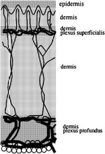
sity F (r¯) and the total radiant-energy-fluence rate U (r)¯ by the MC method [see Eqs. (1.11) and (1.12)], let us represent the skin as a plane multilayer scattering and absorbing medium (Fig. 1.8), with a laser beam falling normally onto its surface. Let us further assume that each ith layer is characterized by the following parameters: μai , μsi , pi (θ), the thickness di , and the refractive index of the filler medium ni . It should be noted that a more general approach to MC simulation that
accounts for the interfaces between the dermal layers as quasi-random periodic surfaces and spectral skin response is also available.243,246
Figure 1.8 A model of human skin.213
Using the MC algorithm described in Refs. 213, 224, 261, and 262 to simulate the distribution of Gaussian light beams in the skin (see Fig. 1.8 and Table 1.1), the total fluence rate at wavelengths 337, 577, and 633 nm was obtained as shown in Fig. 1.9, along with the dependencies of the maximum total radiant-energy-fluence rate U m and the maximum fluence rate area D × D on the incident beam radius r0 at 633 nm (Fig. 1.10). D and D are defined at the 1/e2 level of U along and across the incident light beam, respectively. It is readily seen that the illumination maximum is formed at a certain depth inside the tissue, and the total fluence rate at the point of maximum Um may be significantly higher than that in the middle of the beam incident to the surface of the medium (U0). This was noticed by many authors (see, for instance, Refs. 1, 3, 37, and 210), who emphasized the strong correlation between the Um/U0 ratio and the optical properties of the medium, the incident beam radius, and boundary properties. It appears from Fig. 1.10(b) that an
20 |
Optical Properties of Tissues with Strong (Multiple) Scattering |
Figure 1.9 Results of Monte Carlo simulation of the total radiant-energy-fluence rate distribution U (W/cm2) in skin irradiated by Gaussian laser beams with different wavelengths (λ = 633, 577, and 337 nm), equal radius on the skin surface (r0 = 1.0 mm), and equal intensity at the beam center (U0 = 1 W/cm2).6 z is the linear coordinate (depth inside the skin) and r is the coordinate across the light beam.
Table 1.1 Optical parameters of skin.6,213
N |
Skin layer |
λ, nm |
μa, cm−1 |
μs, cm−1 |
g |
n |
d, μm |
1. |
Epidermis |
337 |
32 |
165 |
0.72 |
1.5 |
100 |
|
|
577 |
10.7 |
120 |
0.78 |
1.5 |
|
|
|
633 |
4.3 |
107 |
0.79 |
1.5 |
|
2. |
Dermis |
337 |
23 |
227 |
0.72 |
1.4 |
200 |
|
|
577 |
3.0 |
205 |
0.78 |
1.4 |
|
|
|
633 |
2.7 |
187 |
0.82 |
1.4 |
|
3. |
Dermis with |
337 |
40 |
246 |
0.72 |
1.4 |
200 |
|
plexus |
577 |
5.2 |
219 |
0.78 |
1.4 |
|
|
superficialis |
633 |
3.3 |
192 |
0.82 |
1.4 |
|
4. |
Dermis |
337 |
23 |
227 |
0.72 |
1.4 |
900 |
|
|
577 |
3.0 |
205 |
0.78 |
1.4 |
|
|
|
633 |
2.7 |
187 |
0.82 |
1.4 |
|
5. |
Dermis with |
337 |
46 |
253 |
0.72 |
1.4 |
600 |
|
plexus |
577 |
6 |
225 |
0.78 |
1.4 |
|
|
profundus |
633 |
3.4 |
194 |
0.82 |
1.4 |
|
|
|
|
|
|
|
|
|
increase in the incident beam radius leads to a broadening of the illuminated area inside the tissue, with the enhancement rate in the transversal direction exceeding that along the beam.
For practical purposes, such calculations for human skin and other multilayered soft tissues are necessary to correctly choose the irradiation doses for photochemical, photodynamic, and photothermal therapy of cancer and many other
Tissue Optics: Light Scattering Methods and Instruments for Medical Diagnosis |
21 |
(a)
(b)
Figure 1.10 Parameters of the maximum illumination area as functions of the incident beam radius. A beam with a Gaussian profile, wavelength 633 nm, power 25 mW. (a) 1, Total illumination in the center of the incident beam U0; 2, maximal total illumination Um; 3, Um/U0.
(b) 1, The size of the maximally illuminated area (at the 1/e2 level) along the beam axis, D ; 2, size of the maximally illuminated area (at the 1/e2 level) across the beam axis D .213
diseases, and the laser coagulation of the superficial blood vessels or transscleral
cyclophotocoagulation.2,3,10–16,22,29,32,33,37,57,72,90,91,210,258–268
In particular, based on the results of MC simulation presented in Figs. 1.9 and 1.10, attenuation of a wide laser beam of intensity I0 at depths z > ld = 1/μeff [see Eq. (1.18)] in a thick tissue may be described as
I (z) ≈ I0bs exp(−μeffz), |
(1.30) |
where bs accounts for additional irradiation of upper layers of a tissue due to backscattering (photon recycling effect). Respectively, the depth of light penetra-
22 |
Optical Properties of Tissues with Strong (Multiple) Scattering |
|
tion into a tissue is |
|
|
|
le = ld[ln bs + 1]. |
(1.31) |
Typically, for tissues bs = 1–5 for beam diameter of 1–20 mm.210,265 Thus, when wide laser beams are used for irradiation of highly scattering tissues with lowabsorption, CW light energy is accumulated in tissue due to the high multiplicity of chaotic long-path photon migrations. A highly scattering medium works as a random cavity, providing the capacity of light energy. The light power density within the superficial tissue layers may substantially (up to fivefold) exceed the incident power density and cause the overdosage during photodynamic therapy or overheating during interstitial laser thermotherapy. On the other hand, the photon recycling effect can be used for more effective irradiation of undersurface lesions at relatively small incident power densities.
1.2 Short pulse propagation in tissues
1.2.1 Basic principles and theoretical background
Based on the time-dependent radiation-transfer theory (RTT), it is possible to analyze the time response of scattering tissue. Such an analysis is important
to provide a |
rationale for |
noninvasive optical |
diagnostic methods |
using |
||
time-resolved |
measurement |
of |
reflectance |
and |
transmittance |
in |
tissues.1,3,31,42,44,71,92,129,130,199,200,203,205,248–254,269–302 In its general form, the
time-dependent RTT equation for time-dependent radiance (or the specific intensity) I (r¯, s,¯ t) can be written as:269,301
|
∂ |
|
|
∂ |
|
|
|
||
|
|
I (r,¯ |
s,¯ t) + |
μtt2 |
|
I (r,¯ s,¯ t) = −μtI (r,¯ s,¯ t) |
|
||
∂S |
∂t |
|
|||||||
+ |
|
t |
)f (t, t |
)dt p(s,¯ s¯ )d . |
(1.32) |
||||
4π 4π −∞ I (r,¯ s¯ , t |
|||||||||
|
|
|
μs |
|
|
|
|
|
|
Compared with the CW equation (1.9), the following notation is introduced into Eq. (1.32): t is time, t2 = l/(μtc) is the average interval between interactions, where c is the velocity of light in the medium; f (t, t ) describes the temporal deformation of a δ-shaped pulse following its single scattering and can be represented in the form of an exponentially decaying function as
|
|
= t1 |
|
− |
t1 |
|
|
|
|
f (t, t |
) |
1 |
exp |
|
t − t |
, |
(1.33) |
||
|
|
|
|
|
|||||
where t1 may be a function of r¯, and t1 is the first moment of the distribution function f (t, t ) that describes the time interval of an individual scattering act at t1 → 0, f (t, t ) → δ(t − t ). The radiance I (r,¯ s,¯ t) in Eq. (1.32) contains two
Tissue Optics: Light Scattering Methods and Instruments for Medical Diagnosis |
23 |
components: the attenuated incident radiation and the diffuse. This equation meets the boundary conditions [see Eq. (1.10)] at (r¯, s)¯ → (r¯, s,¯ t).
When probing the plane-parallel layer of a scattering medium with an ultrashort laser pulse, the transmitted pulse consists of a ballistic (coherent) component, a group of photons having zigzag trajectories, and a highly intensive diffuse component (see Fig. 1.11).1,3,31 Both unscattered photons and photons undergoing forward-directed single-step scattering contribute to the intensity of the ballistic component (composed of photons traveling straight along the laser beam). This component is subject to exponential attenuation with increasing sample thickness [see Eq. (1.1)]. This accounts for the limited utility of ballistic photons for practical diagnostic purposes in medicine.
Figure 1.11 An ultrashort laser pulse propagating through a random medium spreads into a diffuse component, a snake with zigzag paths, and a ballistic component.1
The group of snake photons with zigzag trajectories includes photons that have experienced only a few collisions each. They propagate along trajectories that deviate only slightly from the direction of the incident beam and form the first-arriving part of the diffuse component. These photons carry information about the optical properties of the random medium and parameters of any foreign object that they may happen to come across during their progress.
The diffuse component is very broad and intense since it contains the bulk of incident photons after they have participated in many scattering acts and therefore migrate in different directions and have different path lengths. Moreover, the diffuse component carries information about the optical properties of the scattering medium, and its deformation may reflect the presence of local inhomogeneities in the medium. The resolution obtained by this method at a high light-gathering power is much lower than in the method measuring straight-passing photons. Two probing schemes are conceivable, one recording transmitted photons and the other taking advantage of their backscattering (see Fig. 1.12).
If in the diffusion approximation (valid at μa μs) the tissue is homogeneous and semi-infinite, the size of both the source and the detector is small compared with the distance rsd between them at the tissue surface, and the pulse may be
24 |
Optical Properties of Tissues with Strong (Multiple) Scattering |
Figure 1.12 Typical schemes for time-resolved tissue studies:1 (a) Recording transmitted photons; (b) backscattering regime. A, Probing beam; B, detected radiation. The dark area in the center of the scattering layer is a local inhomogeneity (tumor). Spatial and temporal photon distributions in the medium are shown.
regarded as single; then the light distribution is described by the time-dependent diffusion equation:272,273
2 − cμaD−1 − D−1 |
∂t |
· U (r¯, t) = −Q(r,¯ t), |
(1.34) |
|
∂ |
|
|
which is in fact the generalization of the CW Eq. (1.17). It is worth noting that the diffusion equation is equivalent to the equation for thermal conductivity.286 The
solution of Eq. (1.34) yields the following relation for the number of backscattered photons at the surface for unit time and from unit area R(rsd, t):272,273
|
|
|
|
R(rsd, t) = |
|
|
|
|
z0 |
|
t− |
5/2 |
exp − |
rsd2 + z02 |
exp(−μact), |
|
|
(1.35) |
|||||||||||||||||||
|
|
|
|
|
(4πD)3/2 |
|
|
|
2Dt |
|
|
|
|||||||||||||||||||||||||
and correspondingly for transmittance |
|
|
|
|
|
|
|
|
|
|
|
|
|
|
|
|
|
||||||||||||||||||||
T (r |
|
, d, t) |
= |
(4πD) |
− |
3/2t |
− |
5/2 exp |
−rsd2 |
|
|
(d |
− |
z |
) exp |
(d − z0)2 |
|
|
|
||||||||||||||||||
|
4Dt |
|
|
|
|
||||||||||||||||||||||||||||||||
|
sd |
|
|
|
|
|
|
|
|
|
|
|
|
|
|
|
|
|
0 |
|
|
− |
4Dt |
|
|
|
|||||||||||
|
|
|
|
|
|
− |
(d |
+ |
z |
|
) exp |
|
(d + z0)2 |
|
+ |
(3d |
− |
z ) exp |
− |
(3d − z0)2 |
|
||||||||||||||||
|
|
|
|
|
|
|
|
|
|||||||||||||||||||||||||||||
|
|
|
|
|
|
|
0 |
|
|
|
− |
|
|
4Dt |
|
|
|
|
0 |
|
4Dt |
|
|||||||||||||||
|
|
|
|
|
|
− |
(3d |
+ |
z |
) exp |
− |
(3d + z0)2 |
|
exp( |
|
μ ct), |
|
|
|
(1.36) |
|||||||||||||||||
|
|
|
|
|
|
|
|
|
|
|
|
||||||||||||||||||||||||||
|
|
|
|
|
|
|
|
|
0 |
|
|
|
|
4Dt |
|
|
|
|
|
− |
a |
|
|
|
|
|
|
||||||||||
where z0 |
= |
|
s |
|
|
|
|
|
|
|
|
|
|
|
|
|
|
|
|
|
|
|
|
|
|
|
|
|
|
|
|
|
|
|
|
||
|
(μ )−1, and d is the tissue thickness. |
|
|
|
|
|
|
|
|
|
|
|
|
||||||||||||||||||||||||
In practice, μa and μs |
|
are estimated by fitting Eq. (1.35) or Eq. (1.36) with |
|||||||||||||||||||||||||||||||||||
the shape of a pulse measured by the time-resolved photon counting technique. Experimentally measured optical parameters of many tissues and model media obtained by the pulse method can be found in Refs. 1, 3, 6, 12–15, 31, 88, 89, 129,
Tissue Optics: Light Scattering Methods and Instruments for Medical Diagnosis |
25 |
130, 245, 272–289, and 300. An important advantage of the pulse method is its applicability to in vivo studies owing to the possibility of the separate evaluation of μa and μs using a single measurement in the backscattering or transillumination regimes. It seems appropriate to mention that a search for more adequate approaches to describing tissue responses to laser pulses is underway (see, for instance, Refs. 199, 200, 203, 204, 248–254, and 291–302). Many publications are devoted to image transfer in tissues and the evaluation of the resolving power of
optical tomographic schemes that make use of the first-transmitted photons of ul-
trashort pulses.1,3,71,129,130,245,270,271,279–284,294,297–302
1.2.2Principles and instruments for time-resolved spectroscopy and imaging
The main principle of enhanced viewing through a turbid medium (tissue) using a time-resolved approach is well illustrated in Fig. 1.13.1,31 A contrast image of an object in a scattering medium can be provided by electronic or optical time-
gating of the earliest-arriving, minimally scattered light (ballistic and snake photons), which contains geometric information.1,3,31,71 The typical optical schemes
using the selection of the earliest-arriving photons are presented in Figs. 1.14 and 1.15. The first group of schemes (see Fig. 1.14) uses the electronic time-gating procedure. The time-correlated single-photon-counting technique explores a high- repetition-rate picosecond laser (for example, a cavity-dumped mode-locked dye laser). At the detection of the earliest-arriving photons, the time delay is measured with a time-to-amplitude converter [see Fig. 1.14(a)] and a histogram of the arrival
Figure 1.13 Gated viewing through tissue. An enhanced spatial resolution is obtained by selecting “early” light only.1
26 |
Optical Properties of Tissues with Strong (Multiple) Scattering |
(a)
(b)
Figure 1.14 Techniques for electronically gated viewing.1
times is built up using a large number of low-energy pulses. The time resolution of such a technique is limited to about 50 ps. For more energetic pulses from lasers with a lower repetition rate, the use of streak cameras allows for a time resolution down to 1 ps [see Fig. 1.14(b)]. If a synchroscan streak camera is employed, even a high-repetition rate source with low-energy pulses can be used.
The second group of techniques uses optical nonlinear effects to select photons (see Fig. 1.15).1 For a scheme with an optical Kerr gate, an energetic laser is used. Part of the pulse is transmitted into the tissue and part opens the shutter by use of the optical Kerr effect (the cell with CS2) [see Fig. 1.15(a)]. Since the gate width is determined only by the length of the laser pulse, subpicosecond gate times can be achieved. The Raman-amplifier-gating technique also uses energetic laser pulses. A Stokes wave generated by stimulated Raman scattering in a gas cell is used to probe the tissue [see Fig. 1.15(b)]. The low-intensity transmitted light is amplified in a Raman amplifier, which in turn is pumped by an ultrashort laser pulse. This pulse has the proper time delay to strobe on the desired early temporal part of the light under investigation. The third scheme uses a time-correlated frequencydoubling technique and is often used in optical autocorrelators for monitoring laser pulse characteristics [see Fig. 1.15(c)]. It can be used directly for optical gating of signal photons.
1.2.3 Coherent backscattering
The use of ultrafast laser pulses gives rise to a local peak of intensity backscattered within a narrow solid angle owing to scattered light interference.31,73,74 In
the exact backward direction, the intensity of the scattered light is normally twice
Tissue Optics: Light Scattering Methods and Instruments for Medical Diagnosis |
27 |
(a)
(b)
(c)
Figure 1.15 Gated-viewing technique using nonlinear optical phenomena:1 CS2 is the optical Kerr cell filled by CS2; KDP is the nonlinear crystal for frequency doubling.
the diffuse intensity. Such interference in coherence arises from the time reversal symmetry among various scattered light paths in the backscattering direction. This phenomenon is known as weak localization. The profile of the angular distribution of the coherent peak depends on the transport mean path lt and the absorption coefficient μa. The angular width of the peak is directly related to lt as74
θ ≈ |
λ |
(1.37) |
2πlt . |
In many hard and soft tissues such as human fat tissue, lung cancer tissue, normal and cataractous eye lens, and myocardial, mammary, and dental tissues, the
backscattered coherent peak occurs when the probing laser pulse is shorter than 20 ps.74
28 |
Optical Properties of Tissues with Strong (Multiple) Scattering |
1.3 Diffuse photon-density waves
1.3.1 Basic principles and theoretical background
The frequency-domain (FD) method has been proposed for photon migration studies in scattering media. The method is designed to evaluate the dynamic response of scattered light intensity to modulation of the incident laser beam
intensity in a wide frequency range, usually in tissue research using 50 to
1000 MHz.1,3,4,6,10,52,53,71,129,130,285,286,301–337 The FD method measures the mod-
ulation depth of scattered light intensity mU ≡ acdetector/dcdetector (see Fig. 1.16) and the corresponding phase shift relative to the incident light modulation
Figure 1.16 Schematic representation of the time evolution of the light intensity measured in response to (a) a very narrow light pulse and (b) a sinusoidally intensity-modulated light transversing an arbitrary distance in a scattering and absorbing medium. (a) If the medium is strongly scattering, there are no unscattered components in the transmitted pulse. (b) The transmitted photon density wave retains the same frequency as the incoming wave in the medium. The reduced amplitude of the transmitted wave arises from attenuation related to the scattering and absorption processes. The demodulation is the ratio ac/dc normalized to the modulation of the source.314
Tissue Optics: Light Scattering Methods and Instruments for Medical Diagnosis |
29 |
phase (phase lag). Compared with the time-domain (TD) measurements described earlier, this method is more simple and reliable in terms of data interpretation and immunity from noise. These happen because FD equipment involves amplitude modulation at low peak power, slow rise time [compare Figs. 1.16(a) and 1.16(b)], and hence smaller bandwidths than TD instruments; higher SNRs are attainable as well. Medical FD equipment is more economic and portable, and can be built on the basis of measuring devices used in optical telecommunication systems and studies of optical fiber dispersion.4,328 However, the FD technique suffers from the simultaneous transmission and reception of signals and requires special attempts to avoid unwanted cross talk between the transmitted and detected
signals. The current measuring schemes are based on heterodyning of optical and
transformed signals.1,3,4,6,10,52,53,71,129,130,285–290,301–323,334,335
The development of the theory underlying this method resulted in the discovery of a new type of wave: photon-density waves or waves of progressively decaying intensity. Microscopically, individual photons make random migrations in a scattering medium, but collectively they form a photon-density wave at a modulation frequency ω that moves away from a radiation source (see Figs. 1.16 and 1.17). Diffuse waves of this type are well known in other fields of physics (for example,
thermal waves are excited upon absorption of modulated laser radiation in various media, including biological ones5,6,25). Photon-density waves possess typical wave
properties; e.g., they undergo refraction, diffraction, interference, dispersion, and
attenuation.1,3,4,6,71,52,53,129,130,285,301,303,307–310,313–315,334
(a) |
(b) |
(c) |
Figure 1.17 Schematic representation of photons propagation in scattering media induced by (a) a CW, (b) a pulse, and (c) a sinusoidally intensity-modulated light source.315
In strongly scattering media with weak absorption far from the walls and a source or a receiver of radiation, the light distribution may be regarded as a decaying diffusion process described by the time-dependent diffusion equation for photon density [see Eq. (1.34)]. When a point light source with harmonic intensity modulation is used, placed at the point r¯ = 0,
I (0, t) = I0[1 + mI exp(j ωt)], |
(1.38) |
where mI is the intensity modulation depth of the incident light.
30 |
Optical Properties of Tissues with Strong (Multiple) Scattering |
The solution of Eq. (1.34) for a homogeneous infinite medium can be presented in the form71
U (r¯, t) = Udc(r)¯ + Uac(r,¯ ω) exp(j ωt), |
(1.39) |
|||||||||||
where |
|
|
|
4πDr |
ld |
|
|
|||||
|
|
dc |
= |
|
||||||||
|
U |
|
|
|
I0 |
exp |
−r¯ |
|
, |
(1.40) |
||
|
|
|
¯ |
|
|
|||||||
|
|
|
|
|
|
|
|
|
|
|
||
U |
ac ¯ |
|
) = ˜ac ¯ |
|
exp[− |
|
r |
¯] |
(1.41) |
|||
(r, ω |
|
U (r, ω) |
|
|
ik |
(ω)r , |
||||||
|
|
U |
ω |
) = mI |
I0 |
|
exp |
[− |
k |
ω |
(1.42) |
|
|
4πDr |
|||||||||
|
|
˜ac(r¯, |
|
|
|
i( )r¯], |
|||||
|
|
|
|
|
¯ |
|
|
|
|
|
|
and ω |
= |
2πν is the modulation frequency, l |
d = |
μ−1 |
is the diffusion length [see |
||||||
|
|
|
|
|
|
eff |
|
|
|||
Eq. (1.18)], and kr(ω) and ki(ω) are the real and imaginary parts of the photondensity wave vector, respectively:
k = kr − iki = −i[(μac + iω)/D]0.5, |
(1.43) |
|||||||||||
kr,i = ld−1 |
|
[ |
1 |
+ |
(ωτa)2 |
] |
0.5 |
|
1 |
|
0.5 |
(1.44) |
|
|
|
|
, |
||||||||
|
|
|
2 |
|
|
|
|
|||||
|
|
|
τa−1 = μac, |
|
|
|
|
|
(1.45) |
|||
where τa = 1/(μac) is the average travel time of a photon before being absorbed. An alternating component of this solution is a retreating spherical wave with its center at the point r¯ = 0 that oscillates at a modulation frequency ν and undergoes
a phase shift relative to the phase value at point r¯ = 0 equal to
= kr(ω)r¯. |
(1.46) |
Constant and time-dependent components of the photon-density wave fall with distance as exp(−r/¯ ld) and exp[−ki(ω)r¯], respectively. The length of a photondensity wave is defined by
= |
2π |
= |
2π |
(2cDμa{1 + [1 + (ωτa)2]1/2})1/2, |
(1.47) |
|
kr |
|
ω |
||||

Tissue Optics: Light Scattering Methods and Instruments for Medical Diagnosis |
|
31 |
|||||||||||||||||||||||
and its phase velocity is |
|
|
|
|
|
|
|
|
|
|
|
|
|
|
|
|
|
|
|
|
|||||
|
|
|
|
|
|
|
|
|
V = ν. |
|
|
|
|
|
|
|
(1.48) |
||||||||
It follows that photon-density waves are capable of dispersion. |
|
|
|
|
|
||||||||||||||||||||
|
For biomedical applications, in particular, optical mammography, we can easily |
||||||||||||||||||||||||
|
|
10 |
|
|
|
= |
|
|
|
s |
= |
15 cm−1, μa |
= |
0.035 cm−1 |
, and c |
= |
|||||||||
estimate that for ω/2π |
|
500 MHz, μ |
|
|
|
||||||||||||||||||||
(3 |
× |
10 |
|
9 |
|
|
|
|
|
|
|
= |
|
|
|
|
|
|
|
|
|
|
|
||
= |
/1.33) cm/s; the wavelength is s 5.0 cm and the phase velocity is |
||||||||||||||||||||||||
|
|
× |
10 cm/s. |
|
|
|
|
|
|
|
|
|
|
|
|
|
|
|
|
|
|
|
|
||
Vs 1.77 |
|
|
|
|
|
|
|
|
|
|
|
|
|
|
|
|
|
|
|
|
|
||||
|
For weakly absorbing media, when ωτa 1, |
|
|
|
|
|
|
|
|
|
|||||||||||||||
|
|
|
|
|
|
|
2 |
|
8π2D |
V 2 = 2Dω, |
|
|
|
|
|
|
|
|
|||||||
|
|
|
|
|
|
|
= |
|
; |
|
|
|
|
|
|
(1.49) |
|||||||||
|
|
|
|
|
|
|
ω |
|
|
|
|
|
|
||||||||||||
|
|
mU (r,¯ ω) ≡ ˜Udc¯(r¯) |
= mI exp r¯ |
cμa exp −r¯ |
|
|
|
|
(1.50) |
||||||||||||||||
|
|
|
2D , |
||||||||||||||||||||||
|
|
|
|
Uac(r, ω) |
|
|
|
|
|
|
D |
|
|
|
|
ω |
|
|
|||||||
|
|
|
|
|
|
|
|
|
|
|
|
|
|
|
|
|
0.5 |
|
|
|
|
|
|
|
|
|
|
|
|
|
|
|
(r¯, ω) = r¯ 2D |
|
|
|
|
|
|
(1.51) |
|||||||||||
|
|
|
|
|
|
|
. |
|
|
|
|
|
|
||||||||||||
|
|
|
|
|
|
|
|
|
|
|
|
|
ω |
|
|
|
|
|
|
|
|
|
|
||
It clearly follows from Eq. (1.50) that in order to support the transport of a photondensity wave in a medium, light scattering is needed (see first exponential term); but in contrast, high scattering turns a photon density wave to decay (see second exponential term).
Measuring mU (r¯, ω), (r,¯ ω) allows one to separately determine the transport scattering coefficient μs and the absorption coefficient μa, and evaluate the spatial distribution of these parameters.
1.3.2Principles of frequency-domain spectroscopy and imaging of tissues
Evidently, there is a close relationship between the two time-resolved methods for the assessment of optical properties of tissues. In the case of pulse probing of a scattering medium, Fourier instrumental or computer-aided analysis of scattered pulses
allows us to simultaneously obtain the amplitude-phase response of the medium for a continuous set of harmonics.1,3,4,71,286,301–303,311 Figure 1.18 illustrates the typ-
ical behavior of the amplitude-phase response in a tissuelike phantom (whole or
diluted milk).71 Such characteristics are useful for the spectroscopic examination of tissues, e.g., for in vivo evaluation of hemoglobin oxygenation321,338 or blood glucose level.339–341
The spatial resolution available using photon-density waves is crucial for the visualization of macroinhomogeneities. Theoretical considerations illustrated by

32 |
Optical Properties of Tissues with Strong (Multiple) Scattering |
Figure 1.18 (a) Amplitude and (b) phase responses of a model medium [unskimmed (1, 3) and 40% diluted (2) milk] obtained by the Fourier transformation of experimental pulse responses; 1, 2, recording transmitted pulses, 2-cm-thick cuvette; 3, backscattering regime (large volume of unskimmed milk). The distance between irradiating and detecting optic fibers is rsd = 2 cm.71
Fig. 1.19 for two absorbing macroinhomogeneities in a scattering medium provide
evidence that their separate identification is feasible if the accuracy of the phase and wave amplitude measurements is not less than 1.0 and 2.0%, respectively.310,330
The predicted resolving power of diffuse tomography using photon-density waves is close to 1 mm; i.e., it is comparable to that of positron-emission and magnetoresonance tomography.4,285 Important advantages of optical tomography are technical simplicity, the enhancement of an object’s contrast by molecular dyes, and the visualization of local metabolic processes.
Figure 1.20 presents images of tumor-containing female breast tissue outlined by contour lines for μa and μs that were obtained by exposure to modulated visible and near-IR radiation.71 The tumor is readily discernible because of its high absorption and scattering coefficients.
In principle, a record-breaking resolving power of less than 1 mm can be
achieved by taking advantage of the interference of photon-density waves excited by spaced sources.4,53,302,330,342 Not only a good spatial resolution, but also a high
contrast and low sensitivity to the movements and geometry of the object under
study should be provided to get a high-quality image. A tissue immersion technique can be used to improve image quality.129,324,328 When the imaged tissue
is surrounded with a medium of matched scattering and absorption properties, a uniform transillumination image is obtained and the maximum dynamic range is available to examine variations within the tissue. In addition, it allows one to eliminate the influence of the boundary conditions and geometry for objects with a
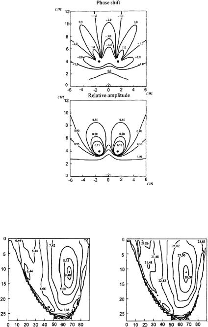
Tissue Optics: Light Scattering Methods and Instruments for Medical Diagnosis |
33 |
Figure 1.19 Theoretical distributions of the relative phase shift and intensity modulation at 200 MHz in an irradiated system of two absolute absorbers (balls 0.5 cm in diameter) placed in a homogeneous scattering medium (μs = 10 cm−1, μa = 0.02 cm−1). The source is located at the origin and the absorbers are located at points (−2, 4) and (2, 4).310
(a) |
(b) |
Figure 1.20 Reconstructed optical images of human cancerous breast tissue obtained by exposure to modulated radiation in the visible and NIR wavelength regions. (a) The image outlined by contour lines for the absorption coefficient μa (10−2 cm−1). (b) The same for the transport scattering coefficient μs (cm−1). The tumor is located near the point (70, 10); the coefficients have relative values.71
34 |
Optical Properties of Tissues with Strong (Multiple) Scattering |
complex shape and structure. It also allows one to achieve optical matching of the probe laser beam and tissue, to considerably reduce the influence of external and internal movements (breathing, heartbeats, muscle tremor, etc.) of the object during the imaging process, and to calibrate measurements using well-known optical properties of the immersion medium. Sometimes, such a simple technique is a good alternative for more sophisticated imaging techniques based on multifrequency analysis.
Apart from the visualization of macroinhomogeneities in breast tissues, the FD method is useful in examining other tissue, e.g., brain and lungs. It also provides an insight into many physiological processes dependent on oxygen consumption by tissues and organs and related hemodynamic changes. One of the most important
areas of application may be the evaluation of the oxygen distribution in a functioning brain.4,285,302,303 Another example is the monitoring of neoplastic growth
patterns, including enhanced blood volume and blood deoxygenation, increased in-
tracellular organelle content, and tissue calcification, which may be important for the differentiation between benign and malignant tumors.285,302,303
To conclude, it should be emphasized that high tissue density sometimes necessitates taking into consideration the time interval of an individual scattering act t1
[see Eqs. (1.32) and (1.33)], which may prove comparable to the mean time interval between interactions t2.301,327 Moreover, the widely used diffusion approximation
imposes important constraints on the analysis of the optical properties of tissues.
Therefore, the development of more universal models of photon-density wave dispersion is well under way using new MC algorithms.301–303,327
1.4 Propagation of polarized light in tissues
1.4.1 Introduction
Up to this point, we have ignored the vector nature of light transport in scattering media such as tissues because we assumed it to be rapidly depolarized during propagation in a randomly inhomogeneous medium. It is a common belief that the randomness of tissue structure results in fast depolarization of light propagating in tissues. Therefore, polarization effects are usually ignored. However, in certain tissues (transparent tissues such as eye tissues, cellular monolayers, mucous membrane, and superficial skin layers), the degree of polarization of transmitted or reflected light remains measurable, even when the tissue has a considerable thickness. In such a situation, the information about the structure of tissues and cell ensembles can be extracted from the registered depolarization degree of initially polarized light, the polarization
state transformation, or the appearance of a polarized component in the scattered
light.3,5,6,59,67–70,105,129,135,138,145,146,148,149,155,159,166,186,343
In regard to practical implications, polarization techniques are believed to give rise to simplified schemes of optical-medical tomography compared with time-
resolved methods, and also provide additional information about the structure of tissues.343–396
Tissue Optics: Light Scattering Methods and Instruments for Medical Diagnosis |
35 |
1.4.2 Tissue structure and anisotropy
Many biological tissues are optically anisotropic.3,9,10,24,29,43,59–70,97,127–130,135, 138,150,151,166,168,176,177,397–440 Tissue birefringence results primarily from the lin-
ear anisotropy of fibrous structures, which forms the extracellular media. The refractive index of a medium is higher along the length of a fiber than along the cross section. A specific tissue structure is a system composed of parallel cylinders that create a uniaxial birefringent medium with the optic axis parallel to the cylinder axes. This is called birefringence of form. A large variety of tissues such as eye cornea, tendon, cartilage, eye sclera, dura mater, testis, muscle, nerve, retina, bone, teeth, myelin, etc. exhibit form birefringence. All of these tissues contain uniaxial and/or biaxial birefringent structures. For instance, in bone and teeth, these are mineralized structures originating from hydroxyapatite crystals, which play an important role in hard tissue birefringence. In particular, dental
enamel is an ordered array of such crystals surrounded by a protein/lipid/water matrix.65,66,97,423,425,426 Fairly well oriented hexagonal crystals of hydroxyapatite
of approximately 30–40 nm in diameter and up to 10 μm in length are packed into an organic matrix to form enamel prisms (or rods) with an overall cross section of 4–6 μm. Enamel prisms are roughly perpendicular to the tooth surface. Tooth dentin is a complex structure, honeycombed with dentinal tubules, which
are shelled organic cylinders with a highly mineralized shell. Tubules diameters are 1–5 μm, and their number density is in the range (3–7) × 106 cm−2.65,66,97,423
Tendon consists mostly of parallel, densely packed collagen fibers arranged
in parallel bundles interspersed with long, elliptical fibroblasts. In general, tendon fibers are cylindrical in shape with diameters ranging from 20 to 400 nm.176,177
The ordered structure of collagen fibers running parallel to a single axis makes tendon a highly birefringent tissue.
Arteries have a more complex structure than tendons. The medial layer consists mostly of closely packed smooth muscle cells with a mean diameter of 15–20 μm. Small amounts of connective tissue, including elastin, collagenous, and reticular fibers, as well as a few fibroblasts, are also located in the media. The outer adventitial layer consists of dense fibrous connective tissue. The adventitia is largely made up of collagen fibers, 1–12 μm in diameter, and thinner elastin fibers, 2–3 μm in diameter. As with tendon, the cylindrical collagen and elastin fibers are ordered mainly along one axis, thus causing the tissue to be birefringent.
Myocardium, on the other hand, contains fibers oriented along two different axes. Myocardium consists mostly of cardiac muscle fibers arranged in sheets that wind around the ventricles and atria. In pigs, the myocardium cardiac muscle is comprised of myofibrils (about 1 μm in diameter) that in turn consist of cylindrical myofilaments (6–15 nm in diameter) and aspherical mitochondria (1–2 μm in di-
ameter). Myocardium is typically birefringent since the refractive index along the axis of the muscle fiber is different from that in the transverse direction.176,177
Form birefringence arises when the relative optical phase between the orthogonal polarization components is nonzero for forward-scattered light. After multiple
36 |
Optical Properties of Tissues with Strong (Multiple) Scattering |
forward scattering events, a relative phase difference accumulates and a delay (δoe) similar to that observed in birefringent crystalline materials is introduced between orthogonal polarization components. For organized linear structures, an increase in phase delay may be characterized by a difference ( noe) in the effective refractive index for light polarized along, and perpendicular to, the long axis of the linear structures. The effect of tissue birefringence on the propagation of linearly polarized light is dependent on the angle between the incident polarization orientation and the tissue axis. Phase retardation δoe between orthogonal polarization components is proportional to the distance d traveled through the birefringent medium:416
δoe = |
2πd noe |
. |
(1.52) |
λ0 |
A medium of parallel cylinders is a positive uniaxial birefringent medium [ noe = (ne − no) > 0] with its optic axis parallel to the cylinder axes [see Fig. 1.21(a)]. Therefore, a case defined by an incident electrical field directed parallel to the cylinder axes will be called “extraordinary,” and a case with the incident electrical field perpendicular to the cylinder axes will be called “ordinary.” The difference (ne − no) between the extraordinary index and the ordinary index is a measure
of the birefringence of a medium comprised of cylinders. For the Rayleigh limit (λ cylinder diameter), the form birefringence becomes399,402
n |
oe = |
(n |
e − |
n |
) |
= |
|
f1f2(n1 − n2)2 |
, |
(1.53) |
|
f1n1 + f2n2 |
|||||||||||
|
|
o |
|
|
|
|
where f1 is the volume fraction of the cylinders; f2 is the volume fraction of the ground substance; and n1, n2 are the corresponding indices. For a given index difference, maximal birefringence is expected for approximately equal volume fractions of thin cylinders and ground material. For systems with large diameter cylinders (λ cylinder diameter), the birefringence goes to zero.402
(a) |
(b) |
Figure 1.21 Models of tissue birefringence: (a) system of long dielectric cylinders, (b) system of thin dielectric plates.442
Tissue Optics: Light Scattering Methods and Instruments for Medical Diagnosis |
37 |
For a system of thin plates [see Fig. 1.21(b)], the following equation is
obtained:160 |
|
|
|
|
|
|
|
n2 |
|
n2 |
|
f1f2(n1 − n2) |
, |
(1.54) |
|
− |
= − f1n12 + f2n22 |
||||||
e |
o |
|
|
||||
where f1 is the volume fraction occupied by the plates; f2 is the volume fraction of the ground substance; and n1, n2 are the corresponding indices. This implies that the system behaves like a negative uniaxial crystal with its optical axis aligned normally with the plate surface.
Form birefringence is used in biological microscopy as an instrument for studying cell structure. The sign of the observed refractive index difference points to the particle shape closest to that of the rod or the plate, and if n1 and n2 are known, one can then assess the volume fraction occupied by the particles. To separate the birefringence of the form and the particle material, the refractive indices of the particles and the ground substance should be matched, because form birefringence vanishes with n1 = n2.
Linear dichroism (diattenuation), i.e., different wave attenuation for two orthogonal polarizations, in systems formed by long cylinders or plates is defined by the difference between the imaginary parts of the effective indices of refraction. Depending on the relationship between the sizes and the optical constants of the cylinders or plates, this difference can take both positive and negative values.160
Reported birefringence values for tendon, muscle, coronary artery, myocardium, sclera, cartilage, and skin are on the order of 10−3 (see, for instance, Refs. 400, 409, 410, and 412–416). The measured refractive index variations for the fast and slow axes of rabbit cornea show that its birefringence varies within the
range of 0 at the apex, or top of the cornea, to 5.5 × 10⁻⁴ at the base of the cornea, where it attaches to the sclera.398,404 The predominant orientation of collagenous
fibers in different regions of the cornea results in birefringence and dichroism.403 Based on experimental results, it has been assumed that the birefringent portions of the corneal surface all have a relatively universal fast axis located approximately 160 deg from the vertical axis, defined as a line that runs from the apex of the cornea through the pupil.404
A new technique—polarization-sensitive optical-coherence tomography (PS
OCT)—allows for the measurement of linear birefringence in turbid tissue with high precision.412–416,418 The following data have been reported using this tech-
nique: for rodent muscle, 1.4 × 10⁻³ (Refs. 415 and 416); for normal porcine tendon, (4.2 ± 0.3) × 10−3 and for thermally treated (90◦C, 20 s), (2.24 ± 0.07) × 10−3; for porcine skin, 1.5 × 10⁻³–3.5 × 10⁻³; for bovine cartilage, 3.0 × 10⁻³ (Ref. 418); and for bovine tendon, (3.7 ± 0.4) × 10−3 (Ref. 413). Such birefringence provides 90% phase retardation at a depth on the order of several hundred micrometers.
The magnitude of birefringence and diattenuation are related to the density and other properties of the collagen fibers, whereas the orientation of the fast axis indicates the orientation of the collagen fibers. The amplitude and orientation of
38 |
Optical Properties of Tissues with Strong (Multiple) Scattering |
birefringence of the skin and cartilage are not as uniformly distributed as in tendon. In other words, the densities of collagen fibers in skin and cartilage are not as uniform as in tendon, and the orientation of the collagen fibers is not distributed in as orderly a fashion.418
In addition to linear birefringence and dichroism (diattenuation), many tissue components show optical activity. In polarized light research, the molecule’s chi-
rality, which stems from its asymmetric molecular structure, results in a number of characteristic effects generically called optical activity.430,434 A well-known man-
ifestation of optical activity is the ability to rotate the plane of linearly polarized light about the axis of propagation. The amount of rotation depends on the chiral molecular concentration, the path length through the medium, and the light wavelength. For instance, chiral asymmetrically encoded in the polarization properties of light transmitted through a transparent media enables very sensitive and accu-
rate determination of glucose concentration. Tissues containing chiral components display optical activity.404,428,429 Interest in chiral turbid media is driven by the
attractive possibility of noninvasive in situ optical monitoring of the glucose in diabetic patients.105,138 Within turbid tissues, however, where the scattering effects
dominate, the loss of polarization information is significant and the chiral effects due to the small amount of dissolved glucose are difficult to detect.
In complex tissue structures, chiral aggregates of particles, in particular spherical particles, may be responsible for optical activity of tissue (see Fig. 1.22). More sophisticated anisotropic tissue models can also be constructed. For example, the cornea can be represented as a system of plane anisotropic layers (plates, i.e., lamellas), each of which is composed of densely packed long cylinders (fibrils) [see Fig. 1.21(a)] with their optical axes oriented along a spiral (see Fig. 2.2). This fibrilar-lamellar structure of the cornea is responsible for the linear and circular dichroism and its dependence on the angle between the lamellas.403
Figure 1.22 Examples of chiral aggregates of spherical particles.
1.4.3 Light scattering by a particle
Let us now consider the transformation of any polarization type (linear, circular, or elliptical) in a scattering medium with typical tissue parameters, and compare the penetration depth of circular and linear polarization in different media. To this end, let us examine a monochromatic plane wave incident on an isolated
Tissue Optics: Light Scattering Methods and Instruments for Medical Diagnosis |
39 |
scatterer.43,148,149 The geometry needed to describe the scattering of light by a particle is shown in Fig. 1.23. The incident monochromatic plane wave comes from below and travels along the positive z-axis. Some of the light is scattered by the
particle along the direction indicated by the vector toward a detector located a
S1
distance r from the particle. The scattering direction is defined by the scattering
angle θ and azimuthal angle ϕ. The scattering plane is originated by the vector
S1 and the z-axis. The electrical field of the incident light is in the x-y plane and can
E |
, and perpendicular, E |
, to the scatter- |
be resolved into components parallel, i |
i |
|
ing plane. The electrical-field vector and the intensity of the incident light beam are given by
i = i + i |
, |
(1.55) |
||
E |
E |
E |
||
Ii = E i E i |
+ E i E i , |
(1.56) |
||
where the asterisk denotes complex conjugation and the angular brackets denote a time average.
Figure 1.23 Geometry of the scattering of light by a particle located at the origin.148 The incident light beam is parallel to the z-axis. A detector is located a distance r from the origin
along the vector .
S1
The electrical field of the scattered light wave is perpendicular to and can
S1
be resolved into components E s and E s , which are parallel and perpendicular,
40 |
Optical Properties of Tissues with Strong (Multiple) Scattering |
respectively, to the scattering plane. The scattered electrical-field vector is given by
s = s + s |
. |
(1.57) |
|
E |
E E |
||
There is a linear relationship between the incident and scattered field components, defined by Eqs. (1.55) and (1.57):43,148,149
E s |
|
eik(r−z) |
S2 |
S3 |
E i |
, |
(1.58) |
|
= |
−ikr |
S4 |
S1 |
|||||
E s |
E i |
|
|
where k = 2π/λ is the wave number, λ = λ0/n¯ is the wavelength in the scatter-
ing medium; n¯ is the mean refractive index of the scattering medium; λ is the
√ 0 wavelength of the light in vacuum; i = −1; r is the distance from the scatterer
to the detector; and z is the position coordinate of the scatterer. The complex num-
bers S1–4 are the elements of the amplitude scattering matrix (S-matrix) or Jones matrix.43,148,149,160,443–449 They each depend on scattering and azimuthal angles θ
and ϕ, and contain information about the scatterer. Both amplitude and phase must be measured to quantify the amplitude scattering matrix. The direct measurements of matrix elements can be done using a two-frequency Zeeman laser, which produces two laser lines with a small frequency separation (about 250 kHz) and orthogonal linear polarizations,149 or by the coherence optical tomography (OCT) technique.418
1.4.4 Polarized light description and detection
Definitions of polarized light and its properties, as well as production and detection techniques, are well described in literature.135,160,443–448 Polarization refers to the
pattern described by the electric-field vector as a function of time at a fixed point in space. When the electrical-field vector oscillates in a single, fixed plane all along the beam, the light is said to be linearly polarized. This linearly polarized wave can be resolved into components parallel and perpendicular to the scattering plane [see Eqs (1.55) and (1.57) and Fig. 1.23]. If the plane of the electrical field rotates, the light is said to be elliptically polarized because the electrical-field vector traces out an ellipse at a fixed point in space as a function of time. If the ellipse happens to be a circle, the light is said to be circularly polarized. The connection between phase and polarization can be understood as follows: circularly polarized light consists of equal amounts of linear mutually orthogonal polarized components that oscillate exactly 90 deg out of phase. In general, light of arbitrary elliptical polarization consists of unequal amplitudes of linearly polarized components, and the electrical fields of the two polarizations oscillate at the same frequency but have some constant phase difference.
Light of arbitrary polarization can be represented by four numbers known as the Stokes parameters, I , Q, U , and V . I refers to the irradiance or intensity of the

Tissue Optics: Light Scattering Methods and Instruments for Medical Diagnosis |
41 |
light; the parameters Q, U , and V represent the extent of horizontal linear, 45 deg linear, and circular polarization, respectively.135,160,443–448
In polarimetry, the Stokes vector S of a light beam is constructed based on six flux measurements obtained with different polarization analyzers in front of the detector:
|
I |
|
|
IH + IV |
|
|
|
S |
Q |
IH − IV |
, |
(1.59) |
|||
|
= U |
= I+45◦ − I−45◦ |
|
|
|
||
|
|
|
|
|
|
|
|
VIR − IL
where IH , IV , I+45◦ , I−45◦ , IR , and IL are the light intensities measured with a horizontal linear polarizer, a vertical linear polarizer, a +45◦ linear polarizer, a −45◦ linear polarizer, a right circular analyzer, and a left circular analyzer in front of the detector, respectively. Because of the relationship IH + IV = I+45◦ + I−45◦ = IR + IL = I , where I is the intensity of the light beam measured without any analyzer in front of the detector, a Stokes vector can be determined by four independent measurements, for example, IH , IV , I+45◦ , and IR :
|
|
|
IH + IV |
|
|
. |
|
||
S = |
2IR |
IH − IV |
|
IV ) |
(1.60) |
||||
|
|
|
(IH |
|
|
|
|
||
|
|
2I+45◦ − (IH |
+ IV ) |
|
|
||||
|
|
− |
|
+ |
|
|
|||
From the Stokes vector, the degree of polarization (DOP), the degree of linear polarization (DOLP), and the degree of circular polarization (DOCP) are derived as
DOP = |
|
Q |
+ I |
+ |
|
, |
|
2 |
U 2 |
|
V 2 |
|
|
Q2 + U 2
DOLP = , (1.61)
I
|
√ |
|
|
|
DOCP = |
V 2 |
. |
||
I |
||||
If the DOP of a light field remains at unity after transformation by an optical system, this system is nondepolarizing; otherwise, the system is depolarizing.
The values of the normalized Stokes parameters, which correspond to a certain type of polarization, are presented in Table 1.2.
The Mueller matrix M of a sample transforms an incident Stokes vector Sin into the corresponding output Stokes vector Sout as
Sout = MSin. |
(1.62) |

42 |
|
Optical Properties of Tissues with Strong (Multiple) Scattering |
||||
|
|
Table 1.2 Polarization types.149 |
|
|
||
|
|
|
|
|
|
|
Stokes |
Horizontal |
Vertical |
+45◦ |
−45◦ |
Right |
Left |
parameter |
(linear) |
(linear) |
(linear) |
(linear) |
(circular) |
(circular) |
|
|
|
|
|
|
|
I |
1 |
1 |
1 |
1 |
1 |
1 |
Q |
1 |
−1 |
0 |
0 |
0 |
0 |
U |
0 |
0 |
1 |
−1 |
0 |
0 |
V |
0 |
0 |
0 |
0 |
1 |
−1 |
Obviously, the output Stokes vector varies with the state of the incident beam, but the Mueller matrix is determined only by the sample and the optical path. Conversely, the Mueller matrix can fully characterize the optical polarization properties of the sample. The Mueller matrix can be experimentally obtained from measurements with different combinations of source polarizers and detection analyzers. In the most general cases, a 4 × 4 Mueller matrix has 16 independent elements; therefore, at least 16 independent measurements must be acquired to determine a full Mueller matrix.
The normalized Stokes vectors for the four incident polarization states, H , V , +45 deg, and R, are, respectively,
|
|
1 |
|
|
|
1 |
|
|
|
|
|
1 |
|
|
|
1 |
|
|
SH i |
1 |
, SV i |
−1 |
, |
S |
45◦i |
0 |
, SRi |
0 |
, (1.63) |
||||||||
|
= |
0 |
|
|
= |
0 |
|
|
+ |
|
= |
0 |
|
|
= |
1 |
|
|
|
|
0 |
|
|
|
0 |
|
|
|
|
|
1 |
|
|
|
0 |
|
|
|
|
|
|
|
|
|
|
|
|
|
where H , V , +45◦, and R, represent horizontal linear polarization, vertical linear polarization, +45 deg linear polarization, and right circular polarization, respectively. We may express the 4 × 4 Mueller matrix as M = [M1 M2 M3 M4], where M1, M2, M3, and M4 are four column vectors of four elements each. The four output Stokes vectors that correspond to the four incident polarization states, H , V , +45 deg, and R, are denoted, respectively, by SH o, SV o, S+45◦o, and SRo. These four output Stokes vectors are experimentally measured based on Eq. (1.60) and can be expressed as
SV o = MSV i = M1 |
− M2 |
. |
(1.64) |
||||||
|
SH o = MSH i = M1 |
+ M2 |
M3 |
|
|||||
S |
45◦o |
|
MS |
45◦i |
|
M1 |
|
||
|
+ |
|
|
+ |
|
|
|
|
|
|
|
|
= |
|
|
= + |
|
|
|
S = MS = M + M
Ro Ri 1 4
The Mueller matrix can be calculated from the four output Stokes vectors as449
M = |
1 |
[SH o + SV o SH o − SV o |
− 2S+45◦ o(SH o + SV o) 2SRo − (SH o + SV o)]. |
(1.65) |
2 |

Tissue Optics: Light Scattering Methods and Instruments for Medical Diagnosis |
43 |
In other words, at least four independent Stokes vectors must be measured to determine a full Mueller matrix, and each Stokes vector requires four independent intensity measurements with different analyzers.
1.4.5 Light interaction with a random single scattering media
In terms of the electrical-field components, the Stokes parameters from Eqs. (1.59) and (1.60) are given by
I = E E + E E |
|
Q = E E − E E . |
(1.66) |
U = E E + E E |
|
V = i(E E − E E )
All Stokes parameters have the same dimension—energy per unit area per unit time per unit wavelength. For an elementary monochromatic plane or spherical electromagnetic wave,145
I 2 ≡ Q2 + U 2 + V 2. |
(1.67a) |
For an arbitrary light beam, as in the case of a partially polarized quasimonochromatic light that is due to the fundamental property of additivity, the Stokes parameters for the mixture of the elementary waves are sums of the re-
spective Stokes parameters of these waves. Equation (1.67a) is replaced by the inequality145,148
I 2 ≥ Q2 + U 2 + V 2. |
(1.67b) |
The degree of polarization (DOP), the degree of linear polarization (DOLP), and the degree of circular polarization (DOCP) for the incident and scattered light are defined by Eq. (1.61). In particular, for the DOLP (PL) and the DOCP (PC ) of the scattered light, we have
|
L = I + I |
= |
|
|
|
Is |
|
|
|||
P |
|
I − I |
|
|
|
Qs2 + Us2 |
, |
(1.68a) |
|||
|
PC = |
|
|
|
|
||||||
|
|
|
|
|
. |
|
|
(1.68b) |
|||
|
|
|
Is s |
|
|
||||||
|
|
|
|
|
V 2 |
|
|
|
|||
In the far field, the polarization of the scattered light is described by the Stokes vector Ss connected with the Stokes vector of the incident light Si [see Eq. (1.62)]148
Ss = M · Si , |
(1.69) |

44 Optical Properties of Tissues with Strong (Multiple) Scattering
where M is the normalized 4 ×4 scattering matrix (intensity or Mueller’s matrix)
|
|
M11 |
M12 |
M13 |
M14 |
. |
|
M |
M21 |
M22 |
M23 |
M24 |
(1.70) |
||
|
= M41 |
M42 |
M43 |
M44 |
|
|
|
|
|
M31 |
M32 |
M33 |
M34 |
|
|
|
|
|
|
|
|
||
Elements of the light-scattering matrix (LSM) depend on the scattering angle θ, the wavelength, and geometrical and optical parameters of the scatterers. M11 is what is measured when the incident light is unpolarized, the scattering angle dependence of which is the phase function of the scattered light. It provides only a fraction of the information theoretically available from scattering experiments.
M11 is much less sensitive to chirality and long-range structure than some of the other matrix elements.148,149 M12 refers to the degree of linear polarization of the
scattered light; M22 displays the ratio of depolarized light to the total scattered light (a good measure of the scatterers’ nonsphericity); M34 displays the transformation of 45-deg obliquely polarized incident light to circularly polarized scattered light (which is uniquely characteristic for different biological systems); the difference between M33 and M44 is a good measure of the scatterers’ nonsphericity.
In addition to the degree of light polarization, defined by Eqs. (1.61), (1.68a), and (1.68b), diattenuation (linear dichroism) is introduced as
DA = |
P12 − P22 |
= |
M122 + M132 + M142 |
, |
(1.71) |
P12 + P22 |
M11 |
where P1 and P2 are the principal coefficients of the amplitude transmission for the two orthogonal polarization eigenstates.
In general, all 16 elements of the LSM are nonzero. However, there are only
seven independent elements (out of 16) in the scattering matrix of a single particle with fixed orientation, and nine relations, which connect the others together.145,146
For scattering by a collection of randomly oriented scatterers, there are 10 independent elements.
The LSM for macroscopically isotropic and symmetric media has the wellknown block-diagonal structure182
|
|
M11(θ) M12(θ) |
|
M(θ) |
M12(θ) M22(θ) |
||
|
= |
0 |
0 |
|
|
0 |
0 |
|
|
|
|
|
0 |
|
0 |
. |
|
|
|
0 |
|
0 |
(1.72) |
||
|
M34 |
(θ) M44 |
(θ) |
|
|
|
M33(θ) |
M34 |
(θ) |
|
|
||
− |
|
|
|
|
|
|
It follows that only eight LSM elements are nonzero and only six of these are
independent. Moreover, there are special relationships for two specific scattering angles 0 and π:145
M22(0) = M33(0), M22(π) = −M33(π),
Tissue Optics: Light Scattering Methods and Instruments for Medical Diagnosis |
45 |
M12(0) = M34(0) = M12(π) = M34(π) = 0, |
(1.73) |
M44(π) = M11(π) − 2M22(π). |
|
Rotationally symmetric particles have an additional property:145 |
|
M44(0) = 2M22(0) − M11(0). |
(1.74) |
The structure of the LSM further simplifies for spherically symmetric particles, which are homogeneous or radially inhomogeneous (composed of isotropic materials with a refractive index that depends only on the distance from the particle center), because in this case145
M11(θ) ≡ M22(θ), M33(θ) ≡ M44(θ). |
(1.75) |
The phase function, i.e., the M11 element, for scattering symmetric relative to the direction of the incident wave depends only on the scattering angle θ and
satisfies the normalization condition [see Eq. (1.14)]145,148 |
|
|
2π 0 |
π M11(θ) sin θdθ = 1, |
(1.76) |
which corresponds to assumption of random distribution of scatterers in a medium. The scattering anisotropy parameter (mean cosine of the scattering angle θ) or the asymmetry parameter of the phase function [see Eq. (1.16)] is expressed now
as
π
g ≡ cos θ = 2π M11(θ) cos θ sin θdθ. (1.77)
0
If a particle is small with respect to the wavelength of the incident light, its scattering can be described as the reemission of a single dipole. This Rayleigh theory is applicable under the condition that m(2πa/λ) 1, where m is the relative
refractive index of the scatterers, (2πa/λ) is the size parameter, a is the radius of the particle, and λ is the wavelength of the incident light in a medium.148 For the
visible and NIR light and scatterers with a typical (for biological tissue) refractive index relative to the ground matter m = 1.05–1.11, the maximum particle radius must be about 12–14 nm for Rayleigh theory to remain valid. For this theory, the scattered irradiance is inversely proportional to λ4 and increases as a6; the angular distribution of the scattered light is isotropic.
The Rayleigh-Gans or Rayleigh-Debye theory addresses the problem of calculating the scattering by a special class of arbitrary shaped particles. It requires
|m − 1| 1 and (2πa /λ)|m − 1| 1, where a is the largest dimension of the particle.129,145,146,149 These conditions mean that the electrical field inside the par-
ticle must be close to that of the incident field and that the particle can be viewed
46 |
Optical Properties of Tissues with Strong (Multiple) Scattering |
as a collection of independent dipoles that are all exposed to the same incident field. A biological cell might be modeled as a sphere of cytoplasm with a higher refractive index (ncp = 1.37) relative to that of the surrounding water medium (nis = 1.35); then m = 1.015, and for the NIR light, this theory is valid for particle dimensions up to a = 0.8–1.0 μm. This approximation has been applied extensively to calculations of light scattering from suspensions of bacteria.149 It can be applicable for describing light scattering from cell components (mitochon-
dria, lysosomes, peroxisomes, etc.) in tissues due to their small dimensions and
refraction.58,96,150–153,163,166
For describing the forward scattering caused by large particles (on the order of 10 μm), the Fraunhofer diffraction approximation is useful.149 According to this theory, the scattered light has the same polarization as that of the incident light and the scatterer pattern is independent of the refractive index of the object. For small scattering angles, the Fraunhofer diffraction approximation can accurately represent the change in irradiance as a function of particle size. That is why this approach is applicable in laser flow cytometry. The structures in a biological cell, such as cell membrane, nuclear texture, and granules in the cytoplasm, can be detected by variations in optical density. An optical Fourier transform of the diffraction pattern can be performed by a lens. Spatial variations in optical density in the object plane are converted by a Fourier transform into spatial frequency variations in the Fourier transform plane in the rear focal plane of the lens.149 If the optical density changes slowly across the object, the Fourier transform places most of the scattered light near zero angles (low spatial frequency) in the Fourier transform plane. This is a good model of a cell with clear cytoplasm (constant optical density). If the optical density changes rapidly across the object, the Fourier transform moves more of the energy to larger scattering angles (higher spatial frequency) in the Fourier transform plane. This is a good model of a cell with highly granular cytoplasm (rapid changes in optical density across the cytoplasm). It was shown that the transforms of abnormal cells have significantly high spatial frequency compared with the transforms of normal cells, in particular single cells in cervical smears. Fourier optical microscopes were developed for such studies. The technique is applicable for a positive photographic transparency of the cell, single cells on slides, and cells in flows.149
Mie or Lorenz-Mie scattering theory is an exact solution of Maxwell’s electromagnetic field equations for a homogeneous sphere.148,160 In the general case,
light scattered at a particle becomes elliptically polarized. For spherically symmetric particles of an optically inactive material, the Mueller scattering matrix is given
by Eqs. (1.72) and (1.75). Mie theory has been extended to arbitrary coated spheres and to arbitrary cylinders.145,146,149 In the Mie theory, the electromagnetic fields of
the incident, internal, and scattered waves are each expanded in a series.160 A lin-
ear transformation can be made between the fields in each of the regions. This approach can also be used for nonspherical objects such as spheroids.145,146 The
linear transformation is called the transition matrix (T-matrix). The T-matrix for spherical particles is diagonal.
Tissue Optics: Light Scattering Methods and Instruments for Medical Diagnosis |
47 |
Thus far, Stokes vectors have been defined for the case of a monochromatic plane wave, and the Mueller matrix for single scattering. These concepts have been generalized to more complicated situations. The Stokes vector was defined for a quasi-monochromatic wave.181 Then in the case of partially polarized light, the inequality, described by Eq. (1.67b), is valid.148
When Mueller matrices from an ensemble of particles differing in size, orientation, morphology, or optical properties are added incoherently, six of the above-
mentioned equalities became inequalities.381 For an ensemble of interacting particles in the single scattering approximation,5,6,10,442 LSM elements have the form
Mij (θ) = Mij0 (θ)NFint(θ), |
(1.78) |
where Mij0 are the LSM elements of an isolated particle, N is the number of scatterers, and Fint(θ) is the interference term, taking into account the spatial correlation of particles. Note that the normalized elements (Mij /M11) in a monodisperse system weakly depend on whether account is taken of the spatial correlation of scatterers, and this ratio is close to that for isolated particles.442
1.4.6 Vector radiative transfer equation
As it was already shown, the majority of tissues are turbid media showing a strong scattering and much less absorption (up to two orders less than scattering in the visible and NIR ranges). Moreover, in their natural state (nonsliced), tissues are
rather thick. Therefore, multiple scattering is a specific feature of a wide class of
tissues.1–3,6,24,31,129,130
Polarization effects at light propagation through various multiply scatter-
ing media, including tissues, are fully described by the vector radiative transfer equation (RTE).59,145,146,188,344–366 The radiative transfer theory (RTT) originated
as a phenomenological approach based on considering the transport of energy through a medium filled with a large number of particles and ensuring energy conservation.182–185 This medium, composed of discrete, sparsely, and randomly distributed particles, is treated as continuous and locally homogeneous. Discussed above, the concept of single scattering and absorption by an individual particle is thus replaced in this subsection by the concept of single scattering and absorption by a small homogeneous volume element. In the framework of the RTT, the scattering and absorption of the small volume element follow from the Maxwell equations and are given by the incoherent sums of the respective characteristics of the constituent particles; the result of scattering is not the transformation of a plane incident wave into a spherical scattered wave but the transformation of the specific
intensity vector (Stokes) of the incident light into the specific intensity vector of the scattered light.146,188
For macroscopically isotropic and symmetric plane-parallel scattering media, the vector radiative transfer equation (VRTE) can be substantially simplified as

48 |
Optical Properties of Tissues with Strong (Multiple) Scattering |
follows:146,188
dS(¯r, ϑ, ϕ) = −S(¯r, ϑ, ϕ) dτ(¯r)
+(¯r) +1 d(cos ϑ ) 2π dϕ Z(¯r, ϑ, ϑ , ϕ − ϕ )S(¯r, ϑ , ϕ ),
4π |
−1 |
0 |
|
(1.79)
where S is the Stokes vector defined by Eq. (1.59); ¯r is the position vector; ϑ, ϕ are the angles characterizing incident direction, respectively, the polar (zenith) and the azimuth angles;
dτ(¯r) = ρ(¯r) σext(¯r) ds |
(1.80) |
is the optical-path-length element, ρ is the local particle-number density, σext is the local ensemble-averaged extinction coefficient, ds is the path-length element measured along the unit vector of the direction of light propagation; is the single scattering albedo; ϑ , ϕ are the angles characterizing scattering direction, respectively, the polar (zenith) and the azimuth angles; Z is the normalized phase matrix
|
¯ |
, ϕ |
− |
ϕ ) |
= |
R( )M(θ)R( ), |
(1.81) |
Z(r, ϑ, ϑ |
|
|
|||||
where M(θ) is the single scattering Mueller matrix, defined by Eq. (1.62); θ is the scattering angle, and R(φ) is the Stokes rotation matrix for angle φ:
|
|
1 |
0 |
0 |
0 |
. |
|
R(φ) |
0 |
cos 2φ |
− sin 2φ |
0 |
(1.82) |
||
|
= |
0 |
0 |
0 |
1 |
|
|
|
|
0 |
sin 2φ |
cos 2φ |
0 |
|
|
|
|
|
|
|
|
Every Stokes vector and Mueller matrix are associated with a specific reference plane and coordinates. In the Mie theory, the Mueller matrix of a single scattering event is defined in the scattering plane that is formed by the incident light vector and the scattered light vector (see Fig. 1.23). For a general coordinate system associated with this scattering plane, the z-axis is along the direction of photon propagation. The x-axis is within the reference plane and is perpendicular to the z-axis. The y-axis is perpendicular to both the z-axis and the reference plane.
There is a local coordinate system associated with each incident photon packet, and its Stokes vector Sin is associated with this local coordinate system. The local coordinate system of the photon before scattering is (x, y, z). After the scattering event, the photon propagates along the z -axis with θ as the polar scattering angle and ϕ as the azimuth angle. The scattering plane is formed by the z-axis and the z -axis, which is the new reference plane.
To calculate the Stokes vector of the scattered light, Eq. (1.59) is used. Because the Mueller matrix of the scattering event defined in the reference plane [see
Tissue Optics: Light Scattering Methods and Instruments for Medical Diagnosis |
49 |
Eq. (1.62)], we need first to transform the Stokes vector of the incident light to the coordinate system associated with the reference plane. This transformation can be done by rotating the local coordinate system (x, y, z) by φ about the z-axis, where the rotation matrix is defined by Eq. (1.82). The new Stokes vector is obtained by
Sin = R(φ)Sin. |
(1.83) |
The local coordinate system of the photon packet is tracked in the process. The transformation can be divided into two steps. The first step is rotating the (x, y, z) system by φ about the z-axis, and the second step is to rotate the coordinate by θ about the rotated y-axis to get (x , y , z ). After the transformation, the z -axis is aligned with the new light vector. The transformation matrix is
x |
= |
cos θ |
0 |
− |
sin θ |
|
cos φ |
sin φ |
0 |
x |
|
y |
0 |
1 |
0 |
− sin φ |
cos φ |
0 |
y . |
(1.84) |
|||
z |
|
sin θ |
0 |
cos θ |
|
0 |
0 |
1 |
y |
|
|
After a photon packet passes through the turbid medium, its Stokes vector is recorded and accumulated. The local coordinate system is tracked in the simulation. In order to record the Stokes vector, the local coordinate system of each photon packet needs to be transformed into the laboratory coordinate system. In the laboratory coordinate system (e1, e2, e3), the local photon coordinate can be written as
x |
e1x |
e2x |
e3x |
e1 |
|
y |
= e1y |
e2y |
e3y |
e2 . |
(1.85) |
z |
e1z |
e2z |
e3z |
e3 |
|
To transform the photon Stokes vector from the local coordinate system into the laboratory coordinate system, the local coordinate system is rotated about its z-axis so that the new x-axis lies within the (e2, e3) plane in the laboratory coordinate. The rotation angle is
φ = tan−1 |
e1y . |
(1.86) |
|
|
|
e1x |
|
The rotation matrix and the new Stokes vector can be obtained from Eqs. (1.82) and (1.83).
The phase matrix, Eq. (1.81), links the Stokes vectors of the incident and scattered beams, specified relative to their respective meridional planes. To compute the Stokes vector of the scattered beam with respect to its meridional plane, one must calculate the Stokes vector of the incident beam with respect to the scattering plane, multiply it by the scattering matrix (to obtain the Stokes vector of the scattered beam with respect to the scattering plane), and then compute the Stokes vector of the scattered beam with respect to its meridional plane. Such a procedure involves two rotations of the reference plane: = −φ; = π − φ and = π + φ;
50 |
Optical Properties of Tissues with Strong (Multiple) Scattering |
and = φ. The scattering angle θ and the angles and are expressed via the polar and the azimuth incident and scattering angles:
cos θ = cos ϑ cos ϑ + sin ϑ sin ϑ cos(ϕ − ϕ),
cos |
= |
cos ϑ − cos ϑ cos θ |
, |
(1.87) |
|
|
|||||
|
sin ϑ sin θ |
|
|||
cos |
= |
cos ϑ − cos ϑ cos θ |
. |
|
|
|
|
||||
|
sin ϑ sin θ |
|
|||
The first term on the right-hand side of the VRTE [Eq. (1.79)] describes the change in the specific intensity vector over the distance ds caused by extinction and dichroism, the second term describes the contribution of light illuminating a small volume element centered at ¯r from all incident directions and scattered into the chosen direction. For real systems, the form of the VRTE tends to be rather complex and often intractable. Therefore, a wide range of analytical and numerical techniques have been developed to solve the VRTE. Because of the important property of the normalized phase matrix, Eq. (1.81), being dependent on the dif-
ference of the azimuthal angles of the scattering and incident directions rather than on their specific values,146,188 an efficient analytical treatment of the azimuthal
dependence of the multiply scattered light, using a Fourier decomposition of the VRTE, is possible. The following techniques and their combinations can be used to solve the VRTE: transfer matrix method, the singular eigenfunction method, the perturbation method, the small-angle approximation, the adding-doubling method,
the matrix operator method, the invariant embedding method, and the Monte Carlo
method.129,138,145,146,187,188,344–368
When the medium is illuminated by unpolarized light and/or only the intensity of multiply scattered light needs to be computed, the VRTE can be replaced by its approximate scalar counterpart. In that case, in Eq. (1.79), the Stokes vector is replaced by its first element (i.e., radiance) [see Eq. (1.9)] and the normalized phase matrix by its (1, 1) element (i.e., the phase function) [see Eq. (1.13)]. The scalar approximation gives poor accuracy when the size of the scattering
particles is much smaller than the wavelength, but provides acceptable results for particles comparable to and larger than the wavelength.146,184 There is ample literature1,3,15,129,130,185,188–190 on the analytical and numerical solutions of the
scalar RTE, Eq. (1.9).
1.4.7 Monte Carlo simulation
The Monte Carlo (MC) method, being widely used for the numerical solution of the RTT equation368–370 in different fields (astrophysics, atmosphere and ocean op-
tics, etc.), appears to be especially promising for the solution of direct and inverse
Tissue Optics: Light Scattering Methods and Instruments for Medical Diagnosis |
51 |
radiation transfer problems for media with arbitrary configurations and boundary
conditions, in particular for the purposes of the medical polarization optical tomography and spectroscopy.1,3,15,41,129,213,215,349,357,361–367 The method is based on the
numerical simulation of photon transport in scattering media. Random migrations of photons inside a sample can be traced from their input until absorption or output occur.
The straightforward simulation using the MC method has the following advantages: (1) one can employ any scattering matrix; (2) there are no obstacles for the use of strongly forward directed phase functions or experimental single scattering matrices; (3) the polarization calculation takes only a twofold increase in computation time over that needed for the evaluation of intensity; (4) any reasonable number of detectors can be accounted for without noticeable increase of the computation time; (5) there are no difficulties in determining the radiation parameters inside the medium; (6) it is possible to model media with complex geometry where radiance depends not only on the optical depth, but also on the transverse coordinates.
The liability of the obtained results to statistical variations on the order of a few percent at an acceptable computation time is the main disadvantage of the MC technique. For a twofold increase of the accuracy, one needs a fourfold increase in the computation time. The MC method is also impractical for great optical depths (τ > 100).
A few MC codes for modeling of polarized light propagation through a scattering layer are available in the literature (see, for example, Refs. 349, 357, and 361–367). To illustrate the MC simulation technique, the algorithm described in Ref. 366 and applied to model the angular dependencies of the scattering matrix elements is discussed. Let a flux of photons within an infinitely narrow beam be incident exactly upon the center of the spherical volume filled up by the scattering particles.366 The path of a single photon migration in the medium is accounted for in a process of computer simulation. The photons are considered in this case as ballistic particles. Different events possible in the course of the photon migration are estimated by the appropriate probability distributions. In the model under study, the photons would either be elastically scattered or absorbed under their collisions with the medium particles. A certain outcome of every event is found by a set of uniformly distributed random numbers. The probability of scattering in the given direction is determined in accordance with scattering by a single particle. One is able to specify the cross section of scattering and values of the scattering matrix elements for every photon interaction with a scatterer.
When an incident photon enters a scattering layer, it is allowed to travel a free path length, l. The l value depends on the particle concentration ρ and extinction cross section σext. The free path length l is a random quantity that takes any positive values with the probability density p(l):
p(l) = ρσexte−ρσextl . |
(1.88) |

52 |
Optical Properties of Tissues with Strong (Multiple) Scattering |
The particular realization of the free path length l is dictated by the value of a random number ξ that is uniformly distributed over the interval [0, 1]:
l
p(l)dl = ξ. |
(1.89) |
0
Substituting Eq. (1.88) into Eq. (1.89) yields the value l of the certain realization in the form
l = − |
1 |
|
ρσext ln ξ. |
(1.90) |
If the distance l is larger than the thickness of the scattering system, then this photon is detected as transmitted without any scattering. If, having passed the distance l, the photon remains within the scattering volume, then the possible events of photon-particle interaction (scattering or absorption) are randomly selected.
Within the spherical system of coordinates, the probability density of photon scattering along the direction specified by the angle of scattering θ between the directions of the incident and scattered photons and by the angle φ between the
previous and new scattering planes is given as |
|
||||
p(θ, φ) = |
|
Is (θ, φ) sin θ |
(1.91) |
||
|
|
|
, |
||
2π |
π |
|
|||
0 |
0 |
Is (θ, φ) sin θdθdφ |
|
||
where Is (θ, φ) is the intensity of the light scattered in the direction (θ, φ) with respect to the previous direction of the photon, defined by angels ϑ and ϕ [see Eqs. (1.79) and (1.80)]. For spherical particles, this intensity is given by the Mie formulas with allowance for the state of polarization of each photon. An integral Is (θ, φ) over all scattering directions, similar to Eq. (1.6), determines the scattering cross section
2π π
σsca = Is (θ, φ) sin θdθdφ. (1.92)
0 0
The probability density of photon scattering along the specified direction, p(θ, φ), depends on the Mueller matrix of the scattering particle M(θ, φ) (a single scattering matrix) and the Stokes vector S associated with the photon [Eqs. (1.59) and (1.69)]. The single scattering Mueller matrix M(θ, φ) links the Stokes vectors of the incident [Si (0, 0)] and scattered [Ss (θ, φ)] light. For spherical scatterers, the elements of this matrix may be factorized:
M(θ, φ) = M(θ)R(φ). |
(1.93) |
The single scattering matrix M(θ) of spherical particles has the form described by Eqs. (1.72) and (1.75). The elements of this matrix are given by the Mie
Tissue Optics: Light Scattering Methods and Instruments for Medical Diagnosis |
53 |
formulas,148,160 which are functions of the scattering angle θ and diffraction parameter x = 2πa/λ, where a is the radius of the spherical particle, and λ is the wavelength in the medium.
The matrix R(φ) describes the transformation of the Stokes vector under rotation of the plane of scattering through the angle φ, which is defined by Eq. (1.82). Thus, the intensity of the light scattered by spherical particles is determined by the expression
Is (θ, φ) = [M11(θ)Ii + (Qi cos 2φ + Ui sin 2φ)M12(θ)], |
(1.94) |
where Qi and Ui are components of the Stokes vector of the incident light [see Eqs. (1.59) and (1.66)]. As it follows from this equation, the probability p(θ, φ) [Eq. (1.91)], unlike the scattering matrix (Eq. 1.93), cannot be factorized, it appears to be parametrized by the Stokes vector associated with the scattered photon. In this case, one should use a rejection method to evaluate p(θ, φ).
The following method of generating pairs of random numbers with the probability density p(θ, φ) may be used.366 In a three-dimensional space, the function p(θ, φ) specifies some surface. The values (θ, φ) corresponding to the distribution p(θ, φ) are chosen using the following steps: (1) a random direction (θξ, φξ) with a uniform spatial distribution is selected, the values of the random quantities θξ, and φξ distributed over the intervals (0, π) and (0, 2π), respectively, are found from the equations
φξ = 2πξ, cos θξ = 2ξ − 1, |
(1.95) |
where ξ is a random number uniformly distributed over the interval (0, 1); (2) the
surface specified by the function p(θ, φ) is surrounded by a sphere of radius R,
equal to the maximum value of the function p(θ, φ), and a random quantity rξ =
ξ R is generated; (3) the direction (θξ, φξ) is accepted as the random direction of the photon scattering at this stage, provided the condition rξ ≤ p(θξ, φξ) is satisfied. In the opposite case, steps 1 and 2 are repeated again.
The migration of the photon in the scattering medium can be described by a sequence of transformations for the related coordinate system. Each scattering event is accompanied by a variation of the Stokes vector associated with the photon. The new Stokes vector Sn+1 is a product of the preceding Stokes vector, transformed to the new scattering plane, and the Mueller matrix Mk(θ) of the scattering particle:
Sn+1 = Mk(θ)Rn(φ)Sn, |
(1.96) |
where the matrix Rn(φ) [see Eq. (1.82)] describes rotation of the Stokes vector around the axis specifying the direction of propagation of the photon before the interaction.
For the chosen scattering direction, the Stokes vector is recalculated using Eqs. (1.69), (1.72), (1.75), and (1.96), and expressions for elements of the singlescattering Mueller matrix for a homogeneous sphere made of an optically inactive
54 |
Optical Properties of Tissues with Strong (Multiple) Scattering |
material.135,148,160 The value thus obtained is renormalized so that the intensity remains equal to unity. Thus, the Stokes vector associated with the photon contains information only about the variation of the state of polarization of the scattered photon. Real intensity is determined by the number of detected photons in the chosen direction within the detector aperture.
The above procedure is repeated as long as the photon appears to be outside the scattering volume. In this case, if the photon propagation direction intersects the surface of the detector, the photon is detected. Upon detection, the Stokes vector is rotated from the current plane of the last scattering to the scattering plane of laboratory coordinate system. The values obtained are accumulated in the appropriate cells of the detector whose number is defined by the photon migration direction. Furthermore, with registering, the photon is classified in accordance with the scattering multiplicity and the length of a total path. For every nonabsorbed photon, the direction and the coordinates of a point at which it escapes the scattering volume, as well as the number of scattering acts it has experienced, were also recorded. The spatial distribution of radiation scattered by the scattering volume can be obtained with regard to polarization by analyzing the above data for a sufficiently great number of photons.
To find the full LSM of an object, one has to detect the light scattering for four linearly independent states of polarization of the incident light, S1i , S2i , S3i , and S4i . This allows one to construct the following system of linear equations:
CM = S , |
(1.97) |
where M is the column matrix composed of matrix elements of the LSM of the object, and S is the 16-element vector containing the Stokes vector elements recorded upon light scattering for the four independent states of the incident light polarization. The transformation matrix C is determined by the choice of the initial set of the Stokes vectors of the incident light. Having solved this system of equations for the set of Stokes vectors, S1i = (1, 1, 0, 0), S2i = (1, −1, 0, 0), S3i = (1, 0, 1, 0), and S4i = (1, 0, 0, 1), one finds the desired LSM of the object, M = M:
|
|
|
|
I1 + I2 |
I1 − I2 |
2I3 − (I1 + I2) |
||||
M |
= |
1 Q1 + Q2 |
Q1 − Q2 |
2Q3 − (Q1 + Q2) |
||||||
|
2 |
|
V1 |
+ V2 |
V1 |
− V2 |
2V3 |
− (V1 |
+ V2) |
|
|
|
|
|
U1 |
U2 |
U1 |
U2 |
2U3 |
(U1 |
U2) |
|
|
|
|
+ |
|
− |
|
− |
+ |
|
2I4 − (I1
2Q4 − (Q1
2U4 − (U1
2V4 − (V1
+I2)
+Q2) ,
+U2)
+V2)
(1.98) where the elements of the Stokes vectors of the scattered light obtained in each of these four cases are denoted as Sn = (In, Qn, Un, Vn), (n = 1, 2, 3, 4). As a result, one may calculate the angular dependencies for all elements of the LSM with allowance for the contributions of multiple scattering.
The simulation was performed for the systems of spherical particles with relative index of refraction m = 1.2, which are uniformly distributed within a spherical volume at volume fraction f = 0.01.366 In the calculations, the illuminating beam was assumed to be infinitely narrow and incident exactly upon the center of the

Tissue Optics: Light Scattering Methods and Instruments for Medical Diagnosis |
55 |
scattering volume in the zero angle direction and the scattered radiation is detected at different scattering angles in the far zone by a detector with the full angular aperture of 1 deg in the scattering plane and 5 deg in a plane that is perpendicular to the scattering one.
The calculated angular distributions of the total scattering intensity for different scattering systems of spherical particles with small radius, a = 50 nm, or large radius, a = 300 nm, are presented in Fig. 1.24. The average multiplicity of scattering of the detected radiation increases with increasing dimensions of the scattering system. For systems of small particles at illumination in the visible range (633 nm), approximation of the Rayleigh scattering is applicable. For rather small dimensions of the scattering volume of 1 mm of diameter, the contribution of single scattering is predominant. This follows from the intensity angular dependence, which is rather isotropic [Fig. 1.24(a)]. As the dimensions of the scattering system increase, the fraction of contributions of the higher multiplicity scattering grows as well. For a 20-mm diameter system, the detected light contains noticeable contributions of scattering of the 10th–20th multiplicity. With a further increase of the system dimensions, most of the incident light is scattered in the backward direction and the scattering intensity in the forward half plane vanishes. For this reason, beginning from a certain value, the dimensions of the scattering system hardly affect the shape of the diagram of the scattering multiplicity distribution.
Figure 1.24 Angular distributions of the total scattering intensity for the multiply scattering systems of spherical particles that have a relative refractive index m = 1.2 and uniformly distributed within a spherical volume at volume fraction f = 0.01: (a) particles with small radius, a = 50 nm, diameter of the system is equal to (1) 1, (2) 2, and (3) 20 mm; and
(b) particles with large radius, a = 300 nm, diameter of the system is equal to (1) 0.002,
(2) 0.2, and (3) 2 mm; the infinitely narrow unpolarized light beam incidents exactly upon the center of the scattering volume in the zero-angle direction (not shown); the wavelength is 633 nm.366
Systems composed of particles with a size on the order of the wavelength [Fig. 1.24(b)] also show an increase in the contributions of higher-order scattering with increasing dimensions of the scattering system. The system transforms
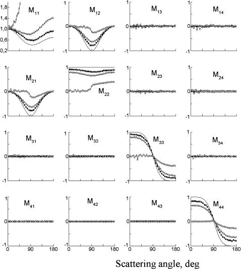
56 |
Optical Properties of Tissues with Strong (Multiple) Scattering |
Figure 1.25 The MC simulation: the angular distributions of the LSM elements for the multiple scattering systems of small spherical particles (a = 50 nm, m = 1.2) uniformly distributed within a spherical volume (f = 0.01); diameter of the system is equal to 1 mm (–"–), 2 mm (–P–), and 20 mm (–!–); the solid line shows the results of calculations in the approximation of single scattering; the infinitely narrow unpolarized light beam incidents exactly upon the center of the scattering volume in the zero-angle direction (not shown); the wavelength is 633 nm.366
from the forward to backward directed scattering mode at rather small thickness, 2-mm diameter.
As it is seen, the intensity of unpolarized light at the higher scattering multiplicity weakly depends on the scattering angle and carries almost no information about the size of the scattering particles. Note that systems of small particles at triple scattering may already be considered as nearly isotropic, while angular dis-
Tissue Optics: Light Scattering Methods and Instruments for Medical Diagnosis |
57 |
Figure 1.26 The MC simulation: the angular distributions of the LSM elements for the multiple scattering systems of large spherical particles (a = 300 nm, m = 1.2) uniformly distributed within a spherical volume (f = 0.01); diameter of the system is equal to 0.002 mm (–"–), 0.2 mm (–P–), and 2 mm (–!–); the solid line shows the results of calculations in the approximation of single scattering; the infinitely narrow unpolarized light beam incidents exactly upon the center of the scattering volume in the zero angle direction (not shown); the wavelength is 633 nm.366
tributions for the large particles, strongly elongated in the forward direction at single scattering, remain anisotropic for sufficiently high scattering multiplicity [four to six scattering events for the system of 0.2 mm diameter, Fig. 1.24(b)].
58 Optical Properties of Tissues with Strong (Multiple) Scattering
The view of the LSM elements’ angular dependences under the conditions of multiple scattering differs substantially from that for the LSM of a single-scattering system. It is seen from Figs. 1.25 and 1.26 that the multiple scattering flattens the angular dependences of the LSM elements. The solid line shows the result of calculation of a normalized LSM for an isolated spherical particle with a similar radius and relative index of refraction. All elements of the LSM are normalized to the M11 element (total scattering intensity) along the given direction, and the element M11 is presented in the plot as normalized to unity in the forward direction; its actual intensity distributions are presented in Fig. 1.24.
Since the single scattering angular distribution for particles with sizes substantially exceeding the Rayleigh limit is strongly asymmetric, the scattering intensity at large angles is very low. For this reason, one must trace the trajectories of a great number of photons to obtain good accuracy in this angular range. Therefore, to
demonstrate the fine structure of the angular dependence of the matrix elements, one needs to use in the simulation 107–108 photons.363,366
For the scattering by particle suspensions in a spherical volume of small diameter, almost all the detected photons are singly scattered. An increase in the optical thickness considerably enhances the contribution of multiple scattering. The angular dependences of the LSM elements have a form close to the single scattering LSM, provided that the optical thickness of the scattering system τ does not exceed unity for the systems of large particles considered ten or above for systems of small particles.
The multiple-scattering intensity (the element M11) for a volume of large diameter decreases with increasing scattering angle slower that the single-scattering intensity. As the cell diameter further increases, the backward scattering becomes predominant (see Figs. 1.24–1.26). In the systems of small particles (see Fig. 1.25), the growth of the multiple scattering contributions is accompanied by a gradual decrease in magnitude of all the elements except for M11; i.e., the form of the LSM approaches that of the ideal depolarizer. In particular, the magnitudes of the elements M12 and M21 decrease in nearly the same way; the elements M33 and M44 also decrease in magnitude, but M44 decreases faster. As a result, multiple scattering gives rise to a difference in the detected values of the elements M33 and M44, even for the systems of spherical particles. The value of the element M22 becomes smaller than unity, this decrease being more substantial in the range of scattering angles close to 90 deg. Thus, the manifestation of the effect of multiple scattering in monodisperse systems of spherical particles, which is revealed in the appearance of nonzero values of the differences |M33 − M44| and |1 − M22|, is similar to the manifestation of the effect of nonsphericity of the scatterers observed under conditions of single scattering.158
For large particle systems, the multiple scattering also decreases the magnitudes and smoothes out the angular dependences of the normalized elements of the LSM (see Fig. 1.26). The corresponding angular dependences, as compared to the LSM of small particles, show the following specific features: the minimum value of the element M22 is reached not at 90 deg, but rather at large scattering angles; the
Tissue Optics: Light Scattering Methods and Instruments for Medical Diagnosis |
59 |
fine structures of the angular dependences for all elements are smeared even in the presence of a small fraction of the multiply scattered light; and, finally, a very important result that the element M44, unlike the other elements, in the limit of high scattering multiplicity, tends to 0.5 rather than to zero for all scattering angles. Such a form of the LSM means that the radiation scattered by the large particles holds the preferential circular polarization at higher scattering multiplicities. This result may serve as a confirmation of preferential survival of different types of polarization
under conditions of multiple scattering for different sizes of scattering particles or tissue structures.59,345,348,438
The process of multiple scattering of the photons during their migration is considered as a series of successive rotations of their coordinate systems, determined by the scattering planes and directions. Since these rotations are random, the detected photons are randomly polarized and, hence, the detected light is partially depolarized. The depolarization will increase with the increasing multiplicity of scattering. For the moderate optical thicknesses (0.2 mm, f = 0.01), the depolarizing ability is strongly different for different directions. The scattered light may be almost completely polarized in the region of small scattering angles, completely depolarized at large angles (θ = 120 deg), and be partly polarized in the backward direction. The angular range of the strongest depolarization corresponds to the angle at which the element M22 acquires minimum values (see Fig. 1.26).
The simulated dependences allow one to estimate the limits of applicability of the single scattering approximation when interpreting the results of experimental studies of disperse scattering systems. It follows from these simulations that modifications of the LSM of monodisperse systems of spherical particles due to the effects of multiple scattering have much in common with modification of the LSM of singly scattering systems upon deviation of the shape of the particles from spherical. This fact imposes serious limitations on the application of the measured LSM of biological objects for the inverse problem solving to determine particle nonsphericity. The appropriate criteria to distinguish the effects of multiple scattering and particle nonsphericity have to be developed.
It is important to note that the comparison of MC simulation accounting for
all orders of multiple scattering with the analytical double-scattering model indicated no essential change in the backscattering polarization patterns.350,351 This is
due to the fact that the main contribution comes from near-double-scattering trajectories in which light suffers two wide-angle scatterings and many near-forward scatterings among multiple-scattering trajectories. The contributions of such multiple but near-double scattering trajectories are obviously well approximated by the contributions of the corresponding double-scattering trajectories.
The above MC technique of photon trajectory modeling is well suited to the simulation of multiple scattering effects in a system of randomly arranged particles. Furthermore, this scheme allows for an approximate approach to describe the interference effects caused by space particle ordering. To this end, one should include the interference of scattered fields into calculations of the single scattering Mueller matrix and integral cross sections for a particle. In other words, at the first
60 |
Optical Properties of Tissues with Strong (Multiple) Scattering |
stage one accounts for the interference effects for simulation of the single scattering properties, and then uses these properties in the MC simulation of multiple scattering. Such an approach is admissible if the size of a region of the local particle ordering is substantially smaller than the mean free-photon path length.
In general, for polarized light propagated in a strongly scattering medium, the multiple scattering decreases the magnitudes and smooths out the angular dependences of the normalized LSM elements, characterizing polarized light interaction with the medium. For media composed of large particles, specified by a high degree of single scattering anisotropy or considerable photon transport length, the scattered radiation holds the preferential circular polarization at higher scattering multiplicities. This theoretical result serves as a confirmation of preferential survival of different types of polarization under conditions of multiple scattering for different sizes of scattering particles or tissue structures.
1.4.8 Strongly scattering tissues and phantoms
Given the known character of the Stokes vector transformation for each scattering act, the state of polarization following multiple light scattering in a highly scattering medium can be found using various approximations of the multiple scattering theory or the MC method. For small particles, the effects of multiple scattering are apparent as the broken symmetry relationship between LSM elements [see Eqs. (1.72)–(1.75)], M12(θ) =M21(θ), M33(θ) =M44(θ), and a significant reduction of linear polarization of the light scattered at angles close to π/2.450
For a system of small spatially uncorrelated particles, the degree of linear (i = L) and circular (i = C) polarization in the far region of the initially polarized
(linearly or circularly) light transmitted through a layer of thickness d is defined by the relation345
Pi = ls |
sinh ξsi exp − |
ξi , |
(1.99) |
||||
|
2d |
|
l |
d |
|
||
where ls = 1/μs is the scattering length, |
|
|
|||||
|
|
ξi = |
ζi ls |
0.5 |
|
(1.100) |
|
|
|
3 |
|
||||
is the characteristic depolarization length for a layer of scatterers, d ξi , ζL = ls /[ln(10/7)], and ζC = ls /(ln 2).
As can be seen from Eq. (1.99), the characteristic depolarization length for linearly polarized light in tissues that can be represented as ensembles of Rayleigh particles is approximately 1.4 times greater than the corresponding depolarization length for circularly polarized light. One can employ Eq. (1.99) to assess the depolarization of light propagating through an ensemble of large-scale spherical particles whose sizes are comparable with the wavelength of incident light (Mie scatter-
ing). For this purpose, one should replace ls by the transport length lt /μ [see
= 1 s
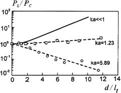
Tissue Optics: Light Scattering Methods and Instruments for Medical Diagnosis |
61 |
Eq. (1.22)] and take into account the dependence on the size of scatterers in ζL and ζC . With the growth in the size of scatterers, the ratio ζL/ζC changes. It decreases from 1.4 down to 0.5 as 2πa/λ increases from 0 up to 4, where a is the radius of scatterers and λ is the wavelength of the light in the medium; it remains virtually constant at the level of 0.5 when 2πa/λ grows from 4 to 15.
Monte Carlo numerical simulations and model experiments in aqueous latex suspensions with particles of various diameters demonstrate that there are three regimes of the dependence of the ratio of the degree of linear polarization to the circular polarization for transmitted light, PL/PC , on d/ lt (Fig. 1.27).345 In the Rayleigh range, PL/PC grows linearly with the increase of d/ lt. In the intermediate range, this ratio remains constant. In the range of Mie scattering, this quantity decreases linearly. Such behavior of this quantity is associated with the transition of the system under study from isotropic scattering to anisotropic scattering. Qualitatively, the physical mechanism behind the change in the depolarization is associated with the fact that a considerable probability of backward scattering in each event of light-medium interaction (isotropic scattering) does not distort linear polarization, whereas backward scattering for circular polarization is equivalent to the reversal of polarization direction (similar to reflection from a mirror), i.e., it is equivalent to depolarization. For the same reason, in the case of a strongly elongated scattering phase function, the degree of circular polarization in an individual scattering event (anisotropic scattering) for light propagating in a layer should remain nonzero for lengths greater than the degree of linear polarization.
Figure 1.27 Semilogarithmic dependencies of the degree of polarization ratio PL/PC on d/ lt for three ka values, k = 2π/λ. The solid line corresponds to Rayleigh scattering (ka 1) and the dashed lines indicate a correspondence between experimental findings and Eq. (1.99) at ls = lt. The experimental points are measurements for aqueous suspensions of polystyrol latex spherical particles having diameter 0.22 (1) and 1.05 (!) μm, where λ0 = 670 nm.345
These arguments also follow from the above MC simulation of polarized light interaction with multiply scattering systems366 and experimental works.429,438 For
example, at high scattering multiplicities the radiation scattered by the large particles holds the preferential circular polarization (LSM element M44 is far from

62 Optical Properties of Tissues with Strong (Multiple) Scattering
zero for all scattering angles, see Fig. 1.26). At multiple scattering, the LSM for a monodisperse system of randomly distributed spherical particles is modified to be approximately identical to the single-scattering LSM of the system containing nonspherical particles, or optically active spheres.366
Thus, different tissues or the same tissues in various pathological or functional states should display different responses to a probe with linearly and circularly polarized light. This effect can be employed in both optical-medical tomography and for determining optical and spectroscopic parameters of tissues. As follows from Eq. (1.99), the depolarization length in tissues should be close to the mean transport path length lt of a photon because this length characterizes the distance within which the direction of light propagation and, consequently, the polarization plane of linearly polarized light becomes totally random after many sequential scattering events.
Since the length lt is determined by the parameter g, characterizing the anisotropy of scattering, the depolarization length should also substantially depend on this parameter. Indeed, the experimental data of Ref. 371 demonstrate that the depolarization length lp of linearly polarized light, which is defined as the length within which the ratio I /I decreases down to 2, displays such a dependence. The ratio mentioned above varied from 300 to 1, depending on the thickness of the sample and the type of tissue (Fig. 1.28). These measurements were performed within a narrow solid angle ( 10−4 sr) in the direction of the incident laser beam. The values of lp differed considerably for the white matter of brain and tissue from the cerebral cortex: 0.19 and 1.0 mm for λ = 476–514 nm and 0.23 and 1.3 mm for λ = 633 nm, respectively. Human skin dermis (bloodless) has a depolarization length of 0.43 mm (λ = 476–514 nm) and 0.46 mm (λ = 633 nm). The depolarization length at λ = 476–514 nm decreases in response to a pathological change
(a) |
(b) |
Figure 1.28 Dependence of the depolarization degree (I /I ) of laser radiation (He:Ne laser, λ = 633 nm; Ar laser, λ = 476/488/514 nm) on the penetration depth for (a) brain tissue (gray and white matter) and (b) whole blood (low hematocrit).371 Measurements were performed within a small solid angle (10−4 sr) along the axis of a laser beam 1 mm in diameter. A strong influence of fluorescence was seen in blood irradiated by the Ar laser.
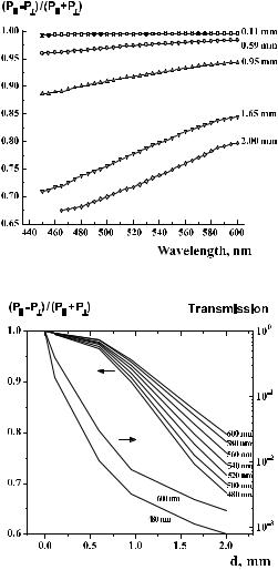
Tissue Optics: Light Scattering Methods and Instruments for Medical Diagnosis |
63 |
in aorta wall tissue: 0.54 mm for normal tissue, 0.39 mm for the stage of tissue calcification, and 0.33 mm for the stage of necrotic ulcer. Whole blood with a low hematocrit is characterized by a considerable depolarization length (about 4 mm) at λ = 633 nm, which is indicative of the dependence on the parameter g, whose
value for blood exceeds the values of this parameter for tissues of many other types, estimated as 0.966–0.997.2,40,48,164
(a) |
(b) |
Figure 1.29 (a) Polarization spectra of light transmitted in the forward direction and (b) the relevant dependencies on the layer thickness d for a gelatin-milk (20%) phantom.374
In contrast to depolarization, the attenuation of collimated light is determined by the total attenuation coefficient μt [see Eq. (1.1)]. For many tissues, μt is much

64 |
Optical Properties of Tissues with Strong (Multiple) Scattering |
greater than μs. Therefore, in certain situations, it is impossible to detect pure bal-
listic photons (photons that do not experience scattering), but the forward-scattered photons retain their initial polarization and can be used for imaging.372,373 This is
illustrated by Figs. 1.29 and 1.30, which present the experimental data for decay
of the degree of linear polarization PL [see Eq. (1.68a)] obtained for a gelatin-milk phantom (a model of bloodless dermis) within a broad wavelength range,77,374 and
for various tissues and blood as a function of light transmission.438 The kink in the characteristics of polarization decay [Fig. 1.29(b)], which can be observed for a small thickness of 0.6 mm, can be attributed to the transition of a medium to the regime of multiple scattering.
Figure 1.30 Degree of linear polarization in different tissues as a function of the sample optical transmittance, Iout/Iin ≡ T , on 633 nm. Each point is an average of three measurements.438 The error bars representing standard deviation of measurements are smaller than the used symbols.
The authors of Ref. 375 experimentally demonstrated that laser radiation re-
tains linear polarization on the level of PL ≤ 0.1 within 2.5lt . Specifically, for skin |
|||||
|
|
|
s |
|
|
irradiated in the red and NIR ranges, we have |
μa |
= |
0.4 cm−1, μ |
= |
20 cm−1, and |
lt = 0.48 mm. Consequently, light propagating in skin can retain linear polariza-
tion within a length of about 1.2 mm. Such an optical path in a tissue corresponds to a time delay on the order of 5.3 ps, which provides an opportunity to produce polarization images of macroinhomogeneities in a tissue with a spatial resolution equivalent to the spatial resolution that can be achieved by the selecting of photons using more sophisticated time-resolved techniques. In addition to the selection of diffuse-scattered photons, polarization imaging makes it possible to eliminate specular reflection from the surface of a tissue, which allows one to use this technique
to image microvessels in facile skin and detect birefringence and optical activity in superficial tissue layers.138,376–378,382,383
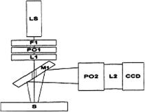
Tissue Optics: Light Scattering Methods and Instruments for Medical Diagnosis |
65 |
Polarization imaging is a new direction in tissue optics.36,129,135,138,344–368, 371–424,428,429,435–442,450,451 The most prospective approaches for polarization tis-
sue imaging, in particular linear-polarization-degree mapping, two-dimensional backscattering Mueller matrix measurements, polarization-sensitive optical coherence tomography (OCT), and a full-field polarization-speckle technique, will be discussed in this and the following chapters.
The registration of two-dimensional polarization patterns for the backscatter-
ing of a polarized incident narrow laser beam is the basis for the polarization imaging technique.375,382,383 The major informative images can be received using the backscattering Mueller matrix approach.351,361–367,380,381,385–387 To determine
each of the 16 experimental matrix elements, a total of 16 images should be taken at various combinations of input and output polarization states.
Figure 1.31 Schematic diagram of the experimental setup for polarization imaging:351,381 LS, 10 mW He:Ne laser (633 nm); F1, 10% neutral density filter; PO1, polarization optics (set 1); L1, focusing lens (f = 10 cm); M1, mirror; S, sample; PO2, polarization analyzer optics (set 2); L2, imaging lens system; CCD, imaging camera.
A schematic view of the experimental setup used for collection of the diffuse backscattered images is shown in Fig. 1.31.351,381 A collimated laser light beam
is polarized via various polarization optics (PO1, linear and circular polarizers) to obtain the desired input polarization. This polarized light is then focused through a hole (about 2 mm in diameter) in a mirror (M1) mounted onto the sample at 45 deg. The diffusely backscattered light from the sample is then imaged through a polarization analyzer (PO2) using a cooled 12-bit CCD camera. The polarization analyzer consists of a variety of optics that were interchanged in order to analyze a specific state of polarization (vertical; horizontal; ±45 deg linear; and left, right circular) for a respective image used to reconstruct the Mueller matrix.
To determine each of the 16 experimental matrix elements, a total of 49 images
(49 − 16 = 33 are dependent) were taken at various combinations of input and output analyzer polarization states.351,381 Each of the 16 experimental elements was
calculated by adding or subtracting a series of images. Each image was collected
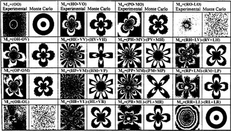
66 |
Optical Properties of Tissues with Strong (Multiple) Scattering |
using an exposure time of 1.7 s, having the speckle effect averaged out (the estimated correlation time of the laser-induced speckles was generally of the order of 10 ms).
A comparison of the measurements of the Mueller matrix elements with the Monte Carlo calculations is presented in Fig. 1.32.351,381 For the MC simulations,
the average number of collisions per photon trajectory was 10. A good agreement between the experimental and calculated patterns, especially azimuthal dependence, can clearly be seen. For the suspensions studied, the transport mean free path lt is about 1 cm. It appears that for distances exceeding two transport mean free paths, the azimuthal dependence of the images becomes less pronounced because multiple scattering tends to randomize the polarization state of the light. It was shown both theoretically and experimentally that only seven matrix elements are independent and the rest can be obtained by simple rotations. The nature of such symmetry is quite general: the scattering medium should be invariant under rotations around the initial laser beam direction and should contain an ensemble (or a
finite number of different ensembles) of identical (possibly asymmetric) scatterers in random orientations.351,381 The polarization images of tissuelike phantoms, can-
cerous and noncancerous cell suspensions, and living tissues (human skin, bone) are presented in Refs. 351, 353–357, 362, and 375–390.
It should be noted that in media containing large-scale scatterers (a common tissue model), depolarization is a higher-order effect ( θ4, θ < 1) than polariza-
Figure 1.32 Experimental and Monte Carlo backscattered Mueller matrix:351,381 The individual images are represented by a two-letter combination that denotes the input polarizer and output analyzer orientation (see Fig. 1.31). HV denotes horizontal input polarized light and a vertical polarization analyzer; V, vertical; H, horizontal; P, +45 deg; M, −45 deg; R, right; L, left; and O, open polarization optics or none. The approximate size of each image is 1.6 × 1.6 cm. The tissuelike phantom was composed of a suspension of 2.02 μm
= |
12 cm−1, g |
= |
0.912, μa |
≈ |
|
polysterene spheres in water: μs |
|
|
0. |
Tissue Optics: Light Scattering Methods and Instruments for Medical Diagnosis |
67 |
tion ( θ2).70 In the literature, the polarization state of multiply scattered light is analyzed either under conditions of spatial diffusion of photons, when the angular spectrum of radiation is virtually isotropic (see, for example, Refs. 184,
393, and 450) or in the case of small-angle scattering in media with large-scale inhomogeneities.70,186,345,450 It should be emphasized, following Ref. 70, that the
analysis of polarization state in the case of small-angular multiple scattering is important for many problems pertaining to optical diagnosis of biological media that
can be represented as random systems with long-range correlation of fluctuations of dielectric permittivity. Such systems display coherent scattering effects73,74,391
or may be expected to show fluctuations of polarization similar to those in disordered media with large-scale inhomogeneities.392–396
In weakly absorbing media that shows a small-angular multiple scattering, the degree of linear polarization for a Henyey-Greenstein phase function [see Eq. (1.15)] is described by the following formula:70
PL = − |
|
2θ2 |
|
1 + |
|
μ z |
|
2 |
− 1 |
2 |
1 + |
μ z |
2 |
. |
(1.101) |
|
|
(μsz)4 |
|
|
|
θ |
|
|
|
θ |
|
|
|||
|
|
|
|
|
|
|
|
|
|
|
|
|
|
|
|
|
|
s |
|
|
s |
|
This means that in a very small angle range (θ μsz), the degree of polarization does not depend on the depth (z)
PL = − |
θ2 |
(1.102) |
8 . |
At the wings of the scattering angle dependence (θ μsz), it tends toward
PL = − |
θ2 |
, |
(1.103) |
2 |
which equals the degree of polarization of singly scattered light.
1.5Optothermal and optoacoustic interactions of light with tissues
1.5.1 Basic principles and classification
The optothermal (OT) method detects the time-dependent heat generated in a tissue via interaction with pulsed or intensity modulated optical radiation.5,6,25,452–518
Such interaction induces a number of thermoelastic effects in a tissue; in par-
ticular, it causes the generation of acoustic waves. The detection of acoustic waves is the basis of optoacoustic (or photoacoustic) methods.5,6,25,455–489,511,512,514–518
The informative features of this method allow one to estimate tissue thermal, optical, and acoustical properties that depend on peculiarities of tissue structure.
Three modes can be used for excitation of tissue thermal response as
follows:5,6,25,455
68 |
Optical Properties of Tissues with Strong (Multiple) Scattering |
(1)A pulse of light (usually pulsed laser) excites the sample and the signal is detected in the time domain with a fast detector attached to a wideband amplifier. In this case, signal averaging and gating techniques are used to increase the SNR.
(2)An intensity-modulated (usually harmonic modulation) light source (highintensity lamp or CW laser) and a low-frequency transducer is used. The measurement is in the frequency domain; phase-sensitive detection (lock- in-amplification of the signal at the modulation frequency) is used for noise suppression.
(3)CW excitation generates a photochemical reaction and the heat evolved through a particular reaction can be detected as a temperature rise.
In every case, the thermal waves generated by the heat release result in several effects that have given rise to various techniques as follows:5,6,25,455
•Optoacoustics (OA) or photoacoustics (PA) (direct or indirect sound wave generation)
•Optothermal radiometry (OTR) or photothermal radiometry (PTR) (detection of infrared thermal emission)
•Photorefractive techniques such as thermal blooming, thermal lensing, probe beam refraction, interferometry, and deflectometry (detection of refractive index gradients above and inside the sample)
•The optogeometric technique (surface deformation in solids, volume changes in fluids)
•Optical calorimetry or laser calorimetry (temperature rise)
The term “optoacoustics” refers primarily to the time-resolved technique utilizing pulsed lasers and measuring the profiles of pressure in tissue; the term “photoacoustics” describes primarily spectroscopic experiments with CW-modulated light and a photoacoustic cell.
A schematic representation of some OT and OA techniques applied to tissue study is given in Fig. 1.33. An excitation laser beam falls onto the sample surface, the light wavelength is tuned to an absorption line of the tissue component of interest, and the optical energy is absorbed by the medium. In a condensed medium, the collisional quenching rate in the component is significantly higher than the radiative rate; therefore, most of the energy transforms to heat. The time-dependent heating leads to all of the above-mentioned thermal and thermoelastic effects. In OA or PA techniques (see 1 in Fig. 1.33), a microphone or a piezoelectric trans-
ducer that is in acoustic contact with the sample is used as a detector to measure the amplitude or phase of the resultant acoustic wave.5,6,455 In the OTR technique
(see 2 in Fig. 1.33), distant IR detectors and array cameras are employed for estimating the temperature of the sample surface and its image.5,6,25,455,490–501 Heating
the medium changes its refractive index. The change in the refractive index of the sample or surrounding gas can be detected either directly by means of an interferometer, or by a probe laser beam that changes its shape, either converging or
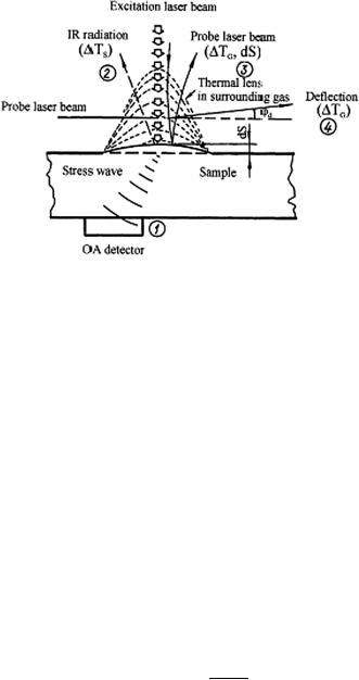
Tissue Optics: Light Scattering Methods and Instruments for Medical Diagnosis |
69 |
Figure 1.33 Schematic representation of some optothermal techniques used in a tissue study:6 TS is the temperature change of a sample; TG is the temperature change of a surrounding gas; dS is the thermoelastic deformation; ϕd is the deflection angle of a probe laser beam. 1, OA technique; 2, OTR technique; 3, thermal lens technique; 4, deflection technique.
diverging (thermal lens, see 3 in Fig. 1.33), or is deflected (see 4 in Fig. 1.33) when it passes the region excited by the pump beam.502–508
The intensity of the signals obtained with any of the OT or OA techniques depends on the amount of energy absorbed and transformed into heat, and on the thermoelastic properties of the sample and its surroundings. Assuming that nonradiative relaxation is the main process in light beam decay and extinction is not very high, μad 1 (d is the length of a cylinder within the sample occupied by a
pulse laser beam), the absorbed energy can be estimated on the basis of Beer’s law
as5,6,25
= |
(1.104) |
ET Eμad, |
where E is the incident pulse energy, and μa is the absorption coefficient.
Energy absorption causes an increase in the local temperature T , which is
defined by the relation5,6,25 |
|
|
|
|
|
T |
|
ET |
Eμad , |
(1.105) |
|
= cP V ρ |
|||||
|
= cP V ρ |
|
|||
where cP is the specific heat capacity for a constant pressure, V = πw2d is the illuminated volume, w is the laser beam radius, and ρ is the medium density. Assuming an adiabatic expansion of an illuminated volume at a constant pressure, one can calculate the change in this volume as
V |
= |
π(w |
+ |
w)2d |
− |
πw2d |
= |
βV T |
βEμad |
, |
(1.106) |
|
|||||||||||
|
|
|
|
= |
cP ρ |
|
|||||
70 |
Optical Properties of Tissues with Strong (Multiple) Scattering |
where w is the change in radius of a cylinder illuminated by a laser beam caused by a local temperature increase and β is the coefficient of volumetric expansion.
This expansion induces a wave propagating in a radial direction with the speed of sound. The corresponding change of pressure p is proportional to the amplitude of mechanical oscillations xT w:
p = 2πfavaρ xT favaρ w, |
(1.107) |
where fa is the frequency of acoustic oscillations and va is the velocity of acoustic waves in a medium.
Using Eq. (1.107) and taking into account that w w, we can finally find:
p |
w |
cP |
Eμa. |
(1.108) |
|
|
|
fa |
βvad |
|
|
Equations (1.105)–(1.108) present the principles of various OT and OA techniques. Information on the absorption coefficient μa at a specific wavelength can be obtained from direct measurements of the temperature change T (optical calorimetry), volume change V (optogeometric technique), or pressure changep (OA and PA techniques). Using the connections between the focal length of the “thermal lens” fT, the deflection angle of a probe laser beam ϕd, and the phase shift in a measuring interferometer ψ with the change in a sample tem-
perature T , the approximate expressions describing the photorefractive methods can be written in the form5,6,25 for a “thermal lens” technique as
fT ≈ dp dT |
w2 |
, |
(1.109) |
|||||
1 |
|
|
|
dn |
|
T |
|
|
a probe beam deflection technique |
n |
dT T , |
|
|||||
ϕd ≈ |
(1.110) |
|||||||
|
|
1 |
|
|
|
dn |
|
|
and a phase shifting (interferometry) technique
ψ ≈ |
λp p |
dT T , |
(1.111) |
|
2πd |
dn |
|
where dn/dT is the medium (tissue) refractive index temperature gradient, dp is the length of the space where the exciting and the probe laser beams are overlapped, and λp is the wavelength of the probe beam.
The effects considered are possible in gases, liquids, and solids. Usually, a tissue under study is surrounded by a gas (composition of gases, like air) or by a liquid (blood, cerebrospinal fluid, aqueous humor, etc.); therefore, a variety of OT

Tissue Optics: Light Scattering Methods and Instruments for Medical Diagnosis |
71 |
and OA effects can be monitored concurrently due to transport of optical intensity, thermal, and acoustic waves in this tissue and its surroundings.5,6,25
The time delay between optical and thermal (acoustic) pulses is an important parameter of the OT (or OA) techniques, defining the SNR. For example, the pulse
OA method can be characterized by the time delay between optical and acoustical pulses as455
= |
(1.112) |
τd Rbd/va, |
where Rbd is the distance between the axis of the exciting laser beam and the acoustic detector.
The time delay for the “thermal lens” technique is defined by the time of the thermal wave propagation transverse to the probing laser beam with a radius wp,455
τth ≈ |
(wp/2.4)2 |
, |
(1.113) |
||
|
aT |
||||
where |
|
|
|
|
|
aT ≈ |
kT |
|
|
(1.114) |
|
ρcP |
|
||||
is the thermal diffusivity of the medium, kT is the heat conductivity, and ρ is the density of the medium. When the duration of a laser pulse τL is much less than τth, focusing the probe laser beam allows one to improve the transit time of this method.
It should be noted that the values of thermal parameters (the heat conductivity kT and the specific heat capacity for a constant pressure cP ) and the density ρ for many tissues are given in Refs. 2 and 87.
1.5.2 Photoacoustic method
For molecular gas systems when the rate of nonradiative relaxation of the excited
states prevails, the time dependent PA signal for excitation by a pulse with the energy E has a form5,6
|
≈ |
|
− |
|
πRG2 |
|
τT |
|
|
δp(t) |
|
(γ |
|
1) |
Eμa |
exp |
−t |
, |
(1.115) |
|
|
|
|
where δp(t) is the time-dependent change in pressure and t is the time; γ = cP /cV and cV is the specific heat capacity for a constant volume; RG is the gas PA cell radius;
τT ≈ |
/2.4)2 |
|
|
(RGaT |
(1.116) |
72 |
Optical Properties of Tissues with Strong (Multiple) Scattering |
|||
is the thermal relaxation time of the PA cell, and |
|
|||
|
aT ≈ |
kG |
(1.117) |
|
|
|
, |
||
|
ρGcV |
|||
where aT |
is defined in Eq. (1.114) for a condensed matter, ρG is the gas density, |
|||
and kG is the gas heat conductivity.
The length of thermal diffusivity (thermal length) is an important parameter,
which for the pulse excitation is estimated as5,6 |
|
lT ≈ (4aT τL)1/2, |
(1.118) |
where τL is the duration of a laser pulse.
Quantitative PA images and spectroscopic studies of tissues can be provided in a frequency-domain mode, when a laser beam of power P intensity modulated at
frequency ω irradiates the sample and the acoustic detector registers the modulation amplitude δp(ω) and the phase lag p(ω) of the acoustic signal.5,6,25,455,460
In that case, the following expressions for δp(ω) and (ω) can be derived:5,6,25 |
|||||
|
|
|
p |
|
|
|
(√ |
|
/2)(γ − 1)(P μa/πRG2 )τT |
|
|
δp(ω) ≈ |
2 |
, |
(1.119) |
||
|
|
[1 + (ωτT )2]1/2 |
|||
p(ω) ≈ − tan−1(ωτT ), |
|
(1.120) |
|||
where τT is defined by Eq. (1.116). These expressions are applicable within the same limits as Eq. (1.115); the notations also coincide with those of Eq. (1.115).
A gas cell PA method is widely seen and used to study optical and thermal properties of condensed materials (liquids and solids).5,6,25,455,457 Light intensity
modulated at frequency ω is absorbed by condensed matter and partially converted into heat, which induces perturbations of the surrounding gas pressure, which in its turn can be registered by a microphone. For a description of the PA signal, three characteristic lengths are usually used: the geometric d, the mean free path
= |
1/μa (when μa |
|
μs), and the “thermal” (thermal diffusion) lT , |
|
of photon lph |
|
|||
|
|
lT = (2aT /ω)1/2, |
(1.121) |
|
where aT is defined by Eq. (1.114) or (1.117), depending on the measuring method used. Six various modes of a gas-microphone method can be used, based on different relations between these three lengths. Evidently for optically and thermally thick samples (d > lT ≈ lph), the PA signal generated can be saturated, and such situations should be avoided.25 For a given sample, lT is defined by modulation frequency ω or pulse duration [see Eq. (1.118)]. For optically and thermally transparent samples (d ≈ lph + lT ), the PA response also includes a back surface of the sample; therefore, besides the six modes mentioned, some others can be used.
Tissue Optics: Light Scattering Methods and Instruments for Medical Diagnosis |
73 |
When light is assumed to be absorbed at the sample surface and heat flow is
approximated by the one-dimensional model, the phase lag can be written in the form460
tan p = tan lT |
|
1 |
+ Rb exp(−2d/ lT ) , |
(1.122) |
||
|
d |
|
1 |
Rb exp( |
2d/ lT ) |
|
|
|
|
|
− |
− |
|
where Rb = (1 − b)/(1 + b), b = (kTbρbcpb/kTρcp)1/2, lT is the thermal diffusion length of tissue [see Eq. (1.121)], and d is the geometric length of the sample (parameters of the backing material are denoted by the subscript b).
Equation (1.122) shows that |
is linear with ω1/2, provided |
p |
|
Rb exp(−2d/ lT ) 1. This condition is generally fulfilled for thermally thick objects (d lT ). However, it is even valid for a thermally thin case if the effusivity of the sample and the backing material are close to each other (b ≈ 1):
p ≈ d/ lT ω1/2. |
(1.123) |
In that case, the images reflect only the thermal diffusivity of the samples. The PA cell was employed in the laser imaging system described in Ref. 460. It has two plane glass windows separated by 1 mm with a silicone sheet spacer. To ensure surface absorption, a sample was covered with copper foil 5-μm thick and placed on the rear window. An intensity-modulated (970 Hz) light beam from an argon laser (200 mW) irradiated the sample from the foil side and was absorbed at its surface. Then, generated heat traveled through the sample and showed the phase lag at the air/sample boundary, which was detected as the PA signal with a microphone. Transparent liquid paraffin was injected between the sample and window to prevent generation of the PA signal on the foil surface. It also worked as a backing material. The sample was embedded in paraffin and sectioned to approximately a 5-μm thick film and placed on copper foil. The observed area of the sample was scanned in increments of 25 μm over 100 × 100 points transverse to a laser beam focused up to 40 μm.
A few types of tissues were studied: a slice of a canine eye and a mouse kidney. From PA phase images, the thermal diffusivity for each point can be obtained. For example, the thermal diffusivity of the optical nerve was estimated as 1.9 × 10⁻⁷ m2/s. The accuracy of the thermal diffusivity measured was about a few tens of percent, primarily due to the difficulty of determining the exact thickness. The calculated thermal diffusion length was about 8 μm. Thus, lateral resolution was limited only by the laser beam diameter and the minimal scanning step. This method may be interesting for examining the relationship between the thermal properties and physiological functions of natural biological microtextures because,
in principle, it requires no fixation. The method belongs to PA microscopy (PAM). The basic principles of PAM are very simple.25,461 Spatially coherent laser ra-
diation serves as a probe beam that can be focused at least to about 1 μm. The scanning of a focused laser beam across the object’s surface and the registration of
74 |
Optical Properties of Tissues with Strong (Multiple) Scattering |
the PA signal induced using a microphone or piezotransducer give the distributions of the optical, thermal, and acoustic properties of the object.
The PAM allows profiling of the object in depth. When the wavelength of the light source is changed, the penetration depth of the light is also changed and the PA signal is generated at different depths. It should also take into account the spectral properties of absorbers and their distribution within the tissue. Another way of depth profiling is to change the modulation frequency. This property is a specific one and characteristic only for PAM. The depth of profiling is defined by the thermal diffusion length of the medium [see Eq. (1.121)] for a given modulation frequency. For example, for a highly absorptive sample (μa ≈ 106 cm−1), a PA signal can be generated at different depths from 10−1 to 103 μm when the modulation frequency is changed in the range from 100 MHz to 1 Hz.
1.5.3 Time-resolved optoacoustics
Measurement of the stress-wave profile and amplitude using an OA spectrometer (see Fig. 1.34), combined with measurement of the total diffuse reflectance, allows one to separately extract both absorption and scattering coefficients of the sample. The absorption coefficient in a turbid medium can be estimated from the acoustic transient profile only if the subsurface irradiance is known. For turbid media irradiated with wide laser beams (> 0.1 mm), the effect of backscattering causes a higher subsurface fluence rate compared with the incident laser fluence (see, for example, Figs. 1.9 and 1.10 for skin). Therefore the z-axial light distribution in tissue and the corresponding stress distribution have a complex profile, with a maximum at a subsurface layer. However, the stress amplitude adjacent to the irradiated surface δp(0) and the stress exponential tail into the depth of the tissue sample can be expressed as467 [see also Eq. (1.30)]
δp(0) = μaE(0), at surface (z = 0), |
(1.124) |
||
1 |
|
|
|
δp(z) = μabsE0 exp(−μeffz), for z > |
|
, |
(1.125) |
μeff |
|||
where = βva2/cT , cT is the specific heat of the tissue, bs is the factor that accounts for the effect of backscattered irradiance that increases the effective energy absorbed in the subsurface layer, μeff is defined in Eq. (1.18), E(0) is the subsurface irradiance, and E0 is the incident laser pulse energy at the sample surface
(J/cm2); the rest of the parameters are given in Eqs. (1.105)–(1.108). For optically thick samples,458,467
E(0) ≈ (1 + 7.1Rd )E0, |
(1.126) |
where Rd is the total diffuse reflection.
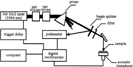
Tissue Optics: Light Scattering Methods and Instruments for Medical Diagnosis |
75 |
The Grüneisen parameter is a dimensionless temperature-dependent factor proportional to the fraction of thermal energy converted into mechanical stress. For water, it can be expressed with an empirical formula (see Ref. 467) as
= 0.0043 + 0.0053T , |
(1.127) |
where temperature T is measured in degrees Celsius; for T = 37◦C ≈ 0.2. Equations (1.124) and (1.125) are strictly valid only when the heating process
is much faster than expansion of the medium. The stress is temporarily confined during laser heat deposition when the duration of the laser pulse is much shorter than the time of stress propagation across the depth of light penetration in the
tissue sample. Such conditions of temporal pressure confinement in a volume of irradiated tissue allow for the most efficient pressure generation.458,459,467
Figure 1.34 Optoacoustic spectrometer for in vitro measurement of optical parameters of tissues:467 SHC, second harmonic converter (532 nm); THC, third harmonic converter (355 nm).
The OA method described and instruments presented in Figs. 1.34 and 1.35
were successfully used for measurement of the optical parameters of some tissues.467,468 The main advantage of this three-wavelengths laser OA spectrometer
for measuring tissue optical properties is the LiNbO3 acoustic detector (Fig. 1.35), which provides high sensitivity ( 100 nV/Pa) combined with a broad ultrasonic frequency range (to 300 MHz) and long-term stability, and thus accurate absolute calibration.467 From OA measurements for human aorta samples (advanced fi- brous atheroma), tissue optical properties were evaluated as μa = 16.5, 3.53, and 0.15 cm−1, and μs = 72.1, 36.5, and 4.85 cm−1, respectively, at wavelengths 355, 532, and 1064 nm for sample thicknesses of 3, 7, and 12 mm, and estimated root- mean-square (rms) values of the measurements, respectively, 10, 15, and 50%. One can measure the absorption and scattering coefficients by using a combination of diffuse reflectance and OA techniques.468 Those measurements at wavelength 1064 nm gave μa = 0.53 ± 0.03 cm−1 and μs = 7.56 ± 0.92 cm−1 for
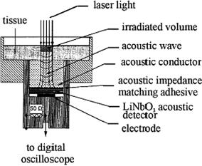
76 |
Optical Properties of Tissues with Strong (Multiple) Scattering |
Figure 1.35 Scheme of an acoustic transducer.467
native canine liver. For coagulated tissue, a 1.3-fold increase in absorption coefficient (μa = 0.71 ± 0.30 cm−1) and a 2.6-fold increase in scattering coefficient (μs = 19.9 ± 6.2 cm−1) were observed. The determination of optical properties of soft tissue in the NIR using OA spectroscopy is also described in Ref. 472. Some data for the optical parameters received using the OA method are given in Table 2.1.
The systematic outline of OA techniques, starting with production and extending to the propagation and detection of OA waves, are presented in Ref. 514. The focal point was the production of acoustic waves with maximal amplitude and minimal distortion. Receiving of the maximal amplitude is important for AO spectroscopy and minimal signal distortion is the key to the determination of optical distribution and imaging in tissues.
1.5.4 Grounds of OA tomography and microscopy
The concept of OA tomography (OAT)458,459,465,466,470,473,475–484 is illustrated in Figs. 1.36 and 1.37. Short laser pulses ensure the temporal confinement of the transient pressure generated in the irradiated volume of tissue as a consequence of laser heating. This means that laser-induced acoustic waves do not move noticeably during laser heating of a tissue volume under study. As a result, the substantial fraction of energy deposited in the target volume (tumor) will generate an ultrasonic wave before it can escape at the speed of sound, and the profile of the laser-induced pressure precisely resembles the distribution of the laser energy absorbed.
If the optical pumping pulse duration is much shorter than the thermal diffusion time, thermal diffusion can be neglected; this is known as the assumption of thermal confinement. In this case, the acoustic wave p(r, t¯), which reaches a detector at position r and time t¯, is related to the optical energy absorption H (r, t¯) by the
Tissue Optics: Light Scattering Methods and Instruments for Medical Diagnosis |
77 |
(a)
(b)
Figure 1.36 Principal schematic diagram of laser OA imaging system for breast cancer diagnostics in (a) transmission mode and (b) temporal pressure profiles recorded upon laser irradiation of the breast phantom with a small “tumor” (the upper profile) and the same profile filtered using a MatLab wavelet transform method.459,465 The x-axis displays the time of transient acoustic wave arrival at the transducer. The “time” axis can be converted into the “depth” axis because depth = time × speed of sound (1.5 mm/μs).
following wave equation:456,517 |
|
|
|
|
|
|
||
|
∂2p(r, t¯) |
− |
2 |
p(r, t¯) = |
βva ∂H (r, t¯) |
, |
(1.128) |
|
|
∂t2 |
|
c |
∂t |
||||
¯ |
|
|
|
T |
¯ |
|
|
|
where t¯ = tva , acoustic speed va is assumed to be constant, H (r, t¯) is the heating function defined as the thermal energy per time and volume deposited by the light

78 |
Optical Properties of Tissues with Strong (Multiple) Scattering |
(a)
(b)
Figure 1.37 Principal schematic diagram of laser OA imaging system for skin cancer diagnostics in (a) reflection mode and (b) OA signals (pressure transients) measured in vivo in tumor tissue (solid line) and normal tissue (dashed line) in a mouse model of breast carcinoma.459,465 During the experiment, tissues were compressed by an attached acoustic transducer; therefore, all depths appear slightly smaller than they actually were.
source in the close proportion to the optical absorption coefficient of interest, and the other parameters are defined earlier. Equation (1.128) can be rewritten in terms of H (r, t¯) as
p(r, t¯) = |
βva |
|
∂H (r , t ) dr |
(1.129) |
|||
|
|
|
|
, |
|||
4πcT |
∂t |
|r − r | |
|||||
where t = t¯− |r− r |. The source term H (r, t¯) can be further rewritten as the product of a purely spatial (optical absorption function) and a purely temporal (function

Tissue Optics: Light Scattering Methods and Instruments for Medical Diagnosis |
79 |
of laser energy) component, i.e., |
|
H (r, t¯) = I0A(r )S(t¯), |
(1.130) |
where I0 is a scaling factor, proportional to the incident radiation intensity; A(r) describes the optical absorption properties of the tissue at r ; and S(t¯) describes the shape of the irradiating pulse. Substituting Eq. (1.130) into (1.131) results in
p(r, t¯) = |
40πcTa |
A(r ) |
dt |
|
) |
|r − r | . |
(1.131) |
|
I βv |
|
dS(t |
|
dr |
|
This equation shows the solution to the forward problem-prediction of the pressure outside the tissue if the absorption properties of the medium and the profile of the laser pulse are known.
For imaging, the inverse problem needs to be solved. Exact inverse solutions in planar, spherical, and cylindrical geometries are available (see references in Ref. 517). These exact solutions are computationally intensive and can be approximated to more efficient solutions in most cases.517 In practice, the distance between the OA sources and the detector is much longer than the wavelength of the high-frequency OA waves that are useful for imaging. Under this condition, the following back-projection algorithm is a good approximate of the inverse solution517
A(r) = C SD |
dSD cos(ϕD ) t |
|
∂t0 |
, t) |
|t=|r0−r|/va , |
(1.132) |
|
|
|
1 |
∂p(r |
|
|
||
|
|
|
|
|
|
|
|
where C is a constant, SD is the surface of detection, and ϕD is the angle between the normal of dSD and r − r0 (the vector pointing from a point of detection to a point of reconstruction).
It should be noted that this is a modified back-projection of the quantity (1/t)[∂p(r0t)/∂t]. This back-projection is analogous to that in x-ray computed tomography (CT). In x-ray CT, the back-projection is along the paths of x-ray propagation; as in OAT, the back-projection is along spherical shells that are centered at the detector and have a radius determined by the acoustic time of flight.
In contrast to photon density waves, acoustic waves (AWs) can provide minimally distorted diagnostic information from sufficient depths in tissue to the surface of a human organ due to their much lower (two to three orders) scatter in tissues than optical waves.517 This is a key point of laser OA imaging and is explained by the independence of its resolution to light scattering. In addition, its low sensitivity to light scattering helps to create more homogeneous light distribution in the volume of diagnostic interest. Light as a carrier of tissue structure information is replaced with a transient AW, which resembles the initial profile of light distribution and can bring this profile to the acoustic detector unaltered. The imaging contrast is based primarily on the optical properties of tissue (absorption), and the imaging resolution is based primarily on the acoustic waves. Wideband ultrasonic detection permits the accurate reproduction of the initial pressure distribution
80 |
Optical Properties of Tissues with Strong (Multiple) Scattering |
in the irradiated volume. Profiles of the pressure transients detected and the time of their arrival carry information on dimensions, optical properties, and location of tumors. Owing to the sensitive detection of AW (5 V/bar), a temperature rise of
only 0.1 mK in a 2-mm tumor located at a depth of 5 cm will be sufficient for the generation of pressure signals with amplitudes of 10 times the noise level.458,459,465
Figures 1.36 and 1.37 present two types of OAT, in a transmission mode and in a reflection mode. The first one can be applied in breast cancer diagnosis and the second one in the detection of skin cancer. A matrix of fiber-optic bundles delivers NIR laser energy from a pulse Nd:YAG laser to the breast surface [see Fig. 1.36(a)]. A matrix of piezoelectric transducers reads temporal profiles of laserinduced acoustic waves. An electronic system digitizes the detected signal profiles and amplifies, filters, and transmits them to a computer for further data processing and image reconstruction. As an example, Fig. 1.36(b) shows a pressure profile recorded for the breast phantom (turbid collagen gel with “tumor” inserted into a 2-mm gel sphere colored with hemoglobin). The bipolar signal that came from a depth of about 5 cm represents a 2-mm spherical “tumor.” The slope of the general pressure profile is due to the exponential decrease in laser energy absorbed in the phantom medium. The normalized and filtered final signal is free of highfrequency noise and other distortions and can be used for image reconstruction. Reconstructed 3D images can be obtained after a minimum of two OA signal matrixes are measured at 90 deg relative to each other.
The reflection-type OAT system contains a fiber-optic light delivery system
with a single piezoelectric transducer, so that AWs can be detected at the site of laser irradiation [see Fig. 1.37(a)].458,459,465 The emphasis in this imaging system is
on high spatial resolution (up to several microns) and therefore the acoustic detector bandwidth must be the widest possible (about 300 MHz). Correspondingly, the laser wavelength and pulse duration should be chosen to generate pressure profiles with a maximum contrast in tissue layers. Figure 1.37(b) shows z-axial profiles of transient pressure signals measured in vivo in a mouse. One mammary gland of the mouse had a tumor (duct carcinoma) located underneath the skin with a diameter of about 5–6 mm and a thickness of about 0.5 mm (histology was performed after the experiments). The tumor had an advanced microcirculation developed as a sphere around it. Two surfaces of the tumor are depicted as two maxima in the OA signal on the axial profile. To obtain 3D images, one needs to scan the OA reflectometer along the area of diagnostic interest. An endoscopic version of the system is possible.
1.5.5 Optothermal radiometry
Pulse laser heating of a tissue causes temperature perturbations and the correspond-
ing modulation of its thermal (infrared) radiation. This is the basis for pulse optothermal radiometry (OTR).491–501 The maximum intensity of the thermal radi-
ation of living objects falls at the wavelength range close to 10 μm. A detailed analysis of OTR signal formation requires knowledge of the internal temperature

Tissue Optics: Light Scattering Methods and Instruments for Medical Diagnosis |
81 |
distribution within the tissue sample, the tissue thermal diffusivity, and its absorption coefficients at the excitation μa and emission μa (10 μm) wavelengths. At the same time, knowledge of some of the parameters mentioned allows one to
use the measured OTR signal to reconstruct, for example, the depth distribution
of μa.491,497
The characteristic thermal time response of a bio object is defined by its dimension R0 (the radius for a cylinder form) and the thermal diffusivity of its material aT [see Eqs. (1.113) and (1.116)] as
τT |
(R0)2 |
(1.133) |
aT . |
Experimental values for the thermal diffusivity aT of some human tissues are presented in Table 1.3. For many soft tissues, these values lie within the rather narrow
range defined by the thermal diffusivity of tissue components: type I hydrated collagen (50% water), 1.03 × 10⁻⁷ m2/s; and pure water, 1.46 × 10⁻⁷ m2/s.494,495
Therefore, the characteristic thermal time response for various organs is mainly
Table 1.3 Experimental values for thermal diffusivity aT of human tissues.2
Tissue |
aT , 10−7 m2/s |
Remarks |
Muscle, underarm |
0.60 |
In vivo, 0.45 mm |
|
1.00 |
In vivo, 0.90 mm |
|
1.30 |
In vivo, 0.90 mm |
Muscle, thigh |
0.545 |
In vivo, 0 . . . 1 mm |
|
0.963 |
In vivo, 1 . . . 2 mm |
Skin |
0.4 . . . 1.6 |
In vivo |
|
0.82 . . . 1.2 |
In vitro, room to body temperature |
Kidney |
1.32 |
In vitro, 5◦C, 84% water |
Heart |
1.48 |
In vitro, 5◦C, 81% water |
Spleen |
1.38 |
In vitro, 5◦C, 80% water |
Liver |
1.50 |
In vitro, 5◦C, 77% water |
Brain |
0.44 . . . 1.4 |
In vitro, room to body temperature |
Brain, white matter |
1.35 |
In vitro, 5◦C, 71% water |
Brain, gray matter |
1.43 |
In vitro, 5◦C, 83% water |
Brain, whole |
1.37 |
In vitro, 5◦C, 78% water |
Blood, hemolyzed |
1.19 |
Power measurement, use of thermal model |
Blood, plasma |
1.21 |
|
Teeth |
4.09 |
– |
|
|
|

82 |
Optical Properties of Tissues with Strong (Multiple) Scattering |
defined by their dimensions and can be estimated as 10−3 s for a cell, 3 × 10⁻² s for a small blood vessel, 102 s for a finger, and more than 104 s for a whole arm.
For a laser pulse duration much shorter than the thermal relaxation time of the sample τT , the normalized to incident radiant exposure and initial temperature OTR signal (the normalized surface temperature) induced in homogeneous absorbing-only and turbid samples is defined by the following expressions derived, respectively, on the basis of Beer’s law and diffusion approximation:497
|
|
|
|
|
|
|
|
|
|
δ |
|
|
|
|
|
|
2 |
|
|
√ |
|
|
|
|
|
|
|
|
|
|
|
√ |
|
|
|
|
|
|
|
|
|
|
|
|
|
|
|
|
|
|
|
|
|
|
|
|
|
|
|
|
|
|
|
|
|
|
|
|
|
|
|
|
|
|
|
|
|
|
|
||||||||
|
Sr (t) = |
|
|
|
|
[exp(δ |
αt)erfc(δ |
αt) |
− δ exp(αt)erfc( |
αt)], |
|
|
|
|
|
(1.134) |
|||||||||||||||||||||||||||
1 − δ2 |
|
|
|
|
|
||||||||||||||||||||||||||||||||||||||
S (t) |
|
|
|
δ 1 − δd2 |
[ |
|
|
|
d |
|
|
|
|
|
|
− |
|
|
|
|
|
|
|
|
|
|
] . |
|
|||||||||||||||
|
|
|
|
|
|
|
|
|
|
|
A |
|
|
exp(δ2 αt)erfc(δd √αt) |
|
|
|
δd exp(αt)erfc(√ |
|
|
) |
|
|
|
|
|
|||||||||||||||||
|
r |
|
|
= |
|
|
|
B |
|
|
|
|
αt |
|
|
|
|
|
|||||||||||||||||||||||||
|
|
|
|
|
|
|
|
|
|
2 |
|
|
|
|
|
|
|
|
|
|
|
|
|
|
|
|
|
|
|
|
|
|
|
||||||||||
|
|
|
|
|
|
|
|
|
|
|
|
|
|
|
|
|
|
|
|
|
√ |
|
|
|
|
|
|
|
|
|
|
√ |
|
|
|
|
|
|
|
||||
|
|
|
|
|
|
|
|
|
|
|
|
|
|
|
exp(δt αt)erfc(δt |
|
αt) |
|
|
δt exp(αt)erfc( |
αt) |
|
|
|
|||||||||||||||||||
|
|
|
|
|
|
|
|
1 − |
δt2 [ |
− |
] |
|
|||||||||||||||||||||||||||||||
|
|
|
|
|
|
|
|
+ |
|
|
|
|
|
|
|
|
|
|
|
|
|
|
|
|
|
|
|
|
|
|
|
|
|||||||||||
|
|
|
|
|
|
|
|
|
|
|
|
|
|
|
|
|
|
|
|
|
|
|
|
|
|
|
|
|
|
|
|
|
|
|
|
|
|
|
|
|
|||
|
|
|
|
|
|
|
|
|
|
|
|
|
|
|
|
|
|
|
|
|
|
|
|
|
|
|
|
|
|
|
|
|
|
|
|
|
|
|
|
|
|
||
|
|
|
|
|
|
|
|
|
|
|
|
|
|
|
|
2 |
|
|
|
|
|
|
|
|
|
|
|
|
|
|
|
|
|
|
|
|
|
|
|
|
|
||
|
|
|
|
|
|
μa/μ , α |
|
|
|
(μ |
|
|
|
|
μd/μ |
|
|
|
|
|
|
|
μ )/μ |
|
|
|
|
|
(1.135) |
||||||||||||||
Here, δ |
= |
= |
) aT , δd |
= |
, δt |
= |
(μa |
+ |
, |
|
erfc(x) |
= |
|||||||||||||||||||||||||||||||
|
|
|
|
− |
|
2 a |
|
|
|
a |
|
|
|
|
|
a |
|
|
|
|
|
|
s a |
|
|
|
|
||||||||||||||||
|
|
|
|
|
|
|
|
|
|
|
|
|
|
|
|
|
|
|
|
|
|
|
|
|
|
|
|
|
|
||||||||||||||
in |
0 |
|
|
|
|
|
|
|
|
|
|
|
|
|
|
|
|
|
|
|
|
|
|
|
|
|
|
|
|
|
|
|
|
|
|
|
|
|
|
||||
|
x e |
|
ξ dξ is the complementary error function, and A and B are defined |
||||||||||||||||||||||||||||||||||||||||
(2/√π) |
|
|
|||||||||||||||||||||||||||||||||||||||||
diffusion theory. The corresponding temperature distributions inside the homogeneous and layered samples are presented in Ref. 497.
The surface radiometric signal Sr (t) at any time t is the sum of the contributions from all depths in the tissue at time t. The radiation from deeper depths is attenuated by the infrared absorption of the sample before reaching the detector. Since the initial surface temperature is known, the temperature distribution into the sample depth can be extracted from the Sr (t) measurement. An inverse OT method to convert surface temperatures as a function of time into internal temperatures as a function of depths is described in Ref. 497.
Figure 1.38 shows the results of pulse OTR experiments conducted on skin using a 577-nm, 1-μs pulsed dye laser.497 Radiometric signals were collected from visibly healthy areas of the wrist and also from a port wine stain on the wrist of a Caucasian volunteer. The laser energy was maintained at 100 mJ over an area of about 20 mm2. The infrared thermal signal from the irradiated area was monitored using a 1-mm2 HgCdTe photoconductive detector with a wavelength detection range of 8 to 12 μm. The detector signal was conditioned using a dc to 1.5 MHz amplifier impedance matched to the detector. The signal was then recorded on a digital oscilloscope. The sampling rate was 10 to 50 μs per point, and 10,000 data points were collected after the laser pulse. The detector response was about 50 mV/◦C. Twenty pulses were averaged to reduce the noise.
The calculated internal temperature distributions for a healthy area on the wrist and for a port wine stain are presented in Figs. 1.38(a) and 1.38(b). There is a noticeable peak in the temperature profile at around 80 μm, indicating a subsurface absorber. The limitations of this technique are that absorption profiles can only be made to a depth of 500 μm before the signal decays too much. Fortunately, most interesting structures in the skin are found between 0 and 600 μm from the skin
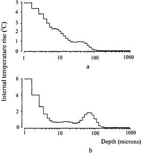
Tissue Optics: Light Scattering Methods and Instruments for Medical Diagnosis |
83 |
Figure 1.38 Depth profiling for skin.497 The graph shows the temperature distribution for
(a) a healthy area of the skin and (b) for a port wine stain. A temperature peak is evident at around 80 μm, indicating the presence of a subsurface absorber.
surface. The uncertainty in the location of the internal temperature layers increases with the depth of the layer.497
However, the single-wavelength pulsed OTR technique is applicable for the accurate determination of port wine stain depth if blood vessels are deeper than 100 μm.498 When blood vessels are close or partially overlap the epidermal melanin layer, a two-wavelength (585 and 600 nm) technique is a superior method to determine lesion depth. It was demonstrated both theoretically and experimentally in in vivo measurements that the two-wavelength method should be appro-
priate for a wider range of port wine stain patients with various blood volume fractions, blood vessel size, and depth distribution.498,499 This is due to the direct-
difference approach used in which vessel depth is determined from a weighted difference of temperature profiles reconstructed independently from two-wavelength measurements.
It was also demonstrated both theoretically and experimentally how morphological information can be extracted from a simplified 2D model of a blood vessel if pulsed OTR imaging is performed and multidimensional analysis of the data is carried out.513
The pulse OTR method has good potentialities in the study of the optical and thermal properties of tissues in vitro and in vivo.490–497 Some data received for
the optical parameters are given in Table 2.1. Sequences (pairs) of infrared emission images recorded following pulsed laser irradiation were used to determine the thermal diffusivity of the biomaterial with a high precision.495 The mean ther-
84 |
Optical Properties of Tissues with Strong (Multiple) Scattering |
mal diffusivity of an in vitro Type I hydrated (50% water) collagen film structure (a model skin phantom) at room temperature (22◦C) deduced from 60 recorded infrared emission image pairs is equal to aT = (1.03 ± 0.07) × 10−7 m2/s. Application of the method to in vivo tissues study was discussed.
The time-resolved OTR was used to determine the absorption coefficients of dental enamel and dentin at 2.79, 2.94, 9.6, and 10.6 μm.454 These data are presented in Table 2.1 and are potentially important in the application of erbium [Er:YSGG (2.79 μm) and Er:YAG (2.94 μm)], or CO2 (9.6 and 10.6 μm) lasers for the ablation of hard dental tissue. On the other hand, the OTR technique may serve for the online monitoring of tooth ablation or hard tissue depth profilometry for the inspection of dental defects.
The frequency-domain OTR technique uses an intensity-modulated laser ra-
diation for inducing modulation frequency-dependent infrared optothermal radiometric (FD-OTR) signals from tissue lesions or defects.500,501 The significance to
dentistry of this technique is caused by its potentiality to monitor dental lesions at the early stages of carious decay where lateral and subsurface spatial resolution on the order of the crack sizes and subsurface depths investigated in Refs. 500 and 501 (100–300 μm) may be required. FD-OTR exhibits a much higher SNR than its pulsed counterpart and a fixed probe depth with the use of a single modulation frequency. For an image to be formed, either the source or the detector must be localized. Photothermal imaging generally falls into the category of scanned microscopy with a localized source. The temperature modulation allows for thermal energy to reach the surface diffusively from a depth approximately equal to a thermal length, described by Eq. (1.118). Scatterers located within a fraction of a thermal length from the source dominate the contrast of radiometric images. In this way, when the thermal length is varied, e.g., by changing the laser beam modulation frequency, the region of the specimen that contributes to the image is also varied.
In dental practice, it is often desirable to obtain detailed local information on potential lesions, and inside pits and fissures with high spatial resolution, such as that achieved with a focused laser source. To meet these objectives, recently a combination of FD-OTR and FD-LUM (luminescence) was used as a fast dental
diagnostic tool to quantify sound enamel or dentin as well as subsurface cracks in human teeth.500,501 Under laser excitation and modulation frequencies in the range
from 10 Hz to 10 kHz, it was found that OTR images are complementary to LUM images as a direct result of the complementary nature of nonradiative (thermal) and radiative (fluorescence) de-excitation processes, which are responsible for the OTR and LUM signal generation, respectively. Measurements were performed at the 488, 659, and 830 nm wavelengths.
A probe beam deflection technique detecting the thermally induced refractive index gradient inside the sample was described [see Eq. (1.110)].502 From the He:Ne laser probe beam deflection measurements and refractive index gradient estimates, it was found that a diode laser (1480 nm) beam produces superheated water of 200◦C. The temperature profile in the diode laser beam and vicinity is predicted as a function of laser pulse duration and power. An optimal (safe) regime to
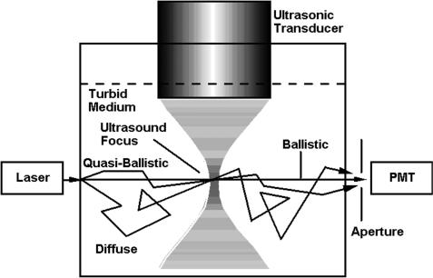
Tissue Optics: Light Scattering Methods and Instruments for Medical Diagnosis |
85 |
dissect the zona pellucida (shell) of preembryos by a focused laser beam (1480 nm) was defined as the pulse duration of ≤5 ms and laser power of 100 mW.
1.5.6 Acoustooptical interactions
Acoustooptical tomography (AOT) or ultrasound-modulated optical tomography
is based on the acoustic [ultrasound (US)] modulation of coherent laser light traveling in tissue.517,519–524 An acoustic wave (AW) is focused into tissue and laser
light is irradiating the same volume within the tissue, for instance, such as it is shown in Fig. 1.39. Any light that is encoded by the ultrasound, including both singly and multiply scattered photons, contributes to the imaging signal. Axial res-
olution along the acoustic axis can be achieved with US-frequency sweeping and subsequent application of the Fourier transformation,517,521 whereas lateral reso-
lution can be obtained by focusing the AW. Three possible mechanisms have been identified for the acoustic modulation of light in scattering tissues517,520,524 (see
Fig. 1.40). The first mechanism is based on US-induced variations of the optical properties of a tissue caused by spatially and temporally dependent tissue compression or rarifying at propagation of the AW. These variations in tissue density cause the corresponding oscillations of tissue optical properties, including absorption and scattering coefficients, and refractive index. Accordingly, the detected intensity of light varies with the AW. However, US modulation of incoherent light has been too weak to be observed experimentally.
The second mechanism is based on variations of the optical properties in response to US-induced displacement of scatterers. The displacements of scatterers,
Figure 1.39 Illustration of the principle of acoustic-modulated optical tomography.520
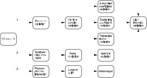
86 |
|
|
|
|
|
|
Optical Properties of Tissues with Strong (Multiple) Scattering |
|||||||||
|
|
|
|
|
|
|
|
|
|
|
|
|
|
|
|
|
|
|
|
|
|
|
|
|
|
|
|
|
|
|
|
|
|
|
|
|
|
|
|
|
|
|
|
|
|
|
|
|
|
|
|
|
|
|
|
|
|
|
|
|
|
|
|
|
|
|
|
|
|
|
|
|
|
|
|
|
|
|
|
|
|
|
|
|
|
|
|
|
|
|
|
|
|
|
|
|
|
|
|
|
|
|
|
|
|
|
|
|
|
|
|
|
|
|
|
|
|
|
|
|
|
|
|
|
|
|
|
|
|
|
|
|
|
|
|
|
|
|
|
|
|
|
|
|
|
|
|
|
|
|
|
|
|
|
|
|
|
|
|
|
|
|
|
|
|
|
|
|
|
|
|
|
|
|
|
|
|
|
|
|
|
|
|
|
|
|
|
|
|
|
|
|
|
|
|
|
|
|
|
|
|
|
|
|
|
|
|
|
|
|
|
|
|
|
|
|
|
|
|
|
|
|
|
|
|
|
|
|
|
|
|
|
|
|
|
|
|
|
|
|
|
|
|
|
|
|
|
|
|
|
|
|
|
|
Figure 1.40 List of possible mechanisms of acoustic modulation of light in tissues.520
assumed to follow AW amplitudes, modulate the physical path lengths of light traveling through the acoustic field. Multiply scattered light accumulates modulated physical path lengths along its path. Consequently, the intensity of the speckles formed by the multiply scattered light fluctuates with the AW. The modulated component of the speckle pattern carries spatial information determined by the US and can be utilized for tomographic imaging.
The third mechanism is caused by photon-phonon interactions, where light is considered as an ensemble of photons and AW—as an ensemble of phonons. The photon-phonon interactions cause a Doppler shift in the classical sense to the frequency of the photons by the acoustic frequency and its harmonics. An optical detector functions as a heterodyning device between the Doppler-shifted light and unshifted light and produces an intensity signal at the acoustic frequency and its harmonics.
Both the second and the third mechanisms require the use of coherent light and both may be associated with the speckle effect. The modulation of the speckles in the second mechanism is caused by the acoustic modulation of scatterer displacements, while the modulation of the speckles in the third mechanism is caused by the acoustic modulation of the refractive index of the tissue. The acoustic modulation of the refractive index also appears in both the first and third mechanisms. However, in the first mechanism, the variation of refractive index causes light that may or may not be coherent to fluctuate in intensity, whereas in the second, the variation of refractive index causes fluctuation in phase of the coherent light, which is converted to fluctuation in intensity by a square-law detector. Thus, as a result of acoustic modulation of the refractive index, the optical phase between two consecutive scattering events is modulated, multiply scattered light accumulates modulated phases along its path, and the modulated phase causes the intensity of the speckles formed by the multiply scattered light to vary with the AW.
Tissue Optics: Light Scattering Methods and Instruments for Medical Diagnosis |
87 |
The intensity modulation depth M is defined as the ratio between the intensity at the fundamental frequency I1 and the unmodulated intensity I0
M = I1/I0. |
(1.136) |
The spectral intensity I1 at fundamental acoustic frequency ωa is calculated from517
1 |
0 |
Ta |
|
|
In = |
|
cos(nωa τ)G1(τ)dτ |
(1.137) |
|
Ta |
||||
at n = 1; here, Ta is the acoustic period. In Eq. (1.137), the autocorrelation function of the scalar electric field, E(t), of the scattered light calculated in the approximation of weak scattering (the optical MFP is much longer than the optical wavelength) and weak modulation (the acoustic amplitude is much less than the optical wavelength) has a view517
G1(τ) = 1 − |
|
6 |
lt ε[1 − cos(ωa τ)], |
(1.138) |
|
|
|
1 |
|
L |
|
where
ε= 6(δn + δd )(n0k0A)2,
δn = (αn1 + αn2)η2,
αn1 = |
ka lt tan−1(ka lt) |
, |
|
|
2 |
|
|||
αn2 = |
|
αn1 |
|
, |
(ka lt)/ tan−1(ka lt) − 1 |
||||
δd = 1 .
6
L is the tissue slab thickness, n0 is the background refractive index, k0 is the optical wave vector in a vacuum, A is the acoustic amplitude, ka is the acoustic wave vector, and lt is the photon transport mean free path. Parameter η is related to the adiabatic piezo-optical coefficient of the tissue ∂n/∂p, the density ρ, and the acoustic velocity va : η = (∂n/∂p)ρ(va )2. The parameters δn and δd (= 1/6) are related to the average contributions per photon free path and per scattering event, respectively, to the ultrasonic modulation of light intensity. The contribution from

88 Optical Properties of Tissues with Strong (Multiple) Scattering
the index of refraction δn increases with ka lt because a longer photon free path, relative to the acoustic wavelength, accumulates a greater phase modulation. By contrast, the contribution from displacement δd stays constant at 1/6, independent of ka and lt. The contribution from the index of refraction above a critical point at ka lt = 0.559, where contributions from refractive index and displacement are equal, increases with ka lt and can significantly outmatch the contribution from displacement.
Accounting for Eq. (1.138), the modulation depth of intensity fluctuations can
be presented as |
|
|
|
|
|
|
1 |
L |
|
2 |
|
M = |
|
lt |
|
ε A2. |
(1.139) |
6 |
This equation shows a quadratic relationship between the intensity modulation depth M and the acoustic amplitude A. Only the nonlinear terms of phase accumulation contribute to the acoustic modulation of coherent light at multiple scattering. The linear term vanishes as a result of optical random walk in scattering media. In the ballistic (nonscattering) regime, M is proportional to A due to nonaveraged contributions from the linear term of phase accumulation. In the quasi-ballistic (minimal scattering) regime, M may show a mixed behavior with A.
It is important to note that the quadratic relationship described by Eq. (1.139) can be experimentally observed if a spectrometer, such as a Fabry-Perot interferometer, is used as a detector. In many cases, the measured modulation depth M is defined as the ratio between the observed ac and dc signals, where the ac signal is originated from the beats between the electric field at the fundamental frequency of the modulated light (ω0 ± ωa ) and the electric field at the intrinsic unmodulated optical frequency (ω0). As a result, the measured modulation depth is approximately described by
M |
I0 |
|
1/2 |
(1.140) |
|
= M1/2 A, |
|||||
|
|
I1 |
|
|
|
indicating that the measured modulation depth is proportional to the acoustic amplitude.
A frequency-swept (chirped) AW is used to encode a laser beam that crosses the acoustic axis of the US transducer with various frequencies.517 Decoding the transmitted light in the frequency domain allows one to image objects buried inside the scattering media. Such images are resolved along the acoustic axis. This encoding scheme is analogous to that of MRI.
A parallel AOT uses a CCD camera for detection of a US-modulated signal pixel by pixel.517 A schematic of the experimental arrangement is shown in Fig. 1.41(a). The z-axis is on the acoustic axis pointing from the US transducer to the sample, the y-axis is along the optical axis pointing to the diode laser, and the x-axis is perpendicular to both the acoustic and optical axes. The AOT system, described in Ref. 517, had the following parameters: a focused US transducer
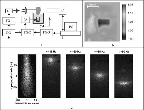
Tissue Optics: Light Scattering Methods and Instruments for Medical Diagnosis |
89 |
Figure 1.41 Parallel AOT.517 (a) Schematic of the experimental setup: DL, diode laser; C, CCD camera; U, ultrasonic transducer; FG-1, FG-2, and FG-3, function generators; DG, delay generator; PA, power amplifier; T, tissue sample. (b) Experimental two-dimensional image of 1.2-cm-thick chicken breast tissue containing a buried object; the horizontal and vertical axes are along the x- and z-axes, respectively. (c) Demonstration of the virtual source of ultrasound-modulated light; left frame, the entire virtual source; following frames, virtual sources corresponding to various values of y obtained by adjusting the frequency fh.
with a 2.54-cm focal length in water, a 1-MHz central response frequency, and the peak focal pressure of 2 × 10⁵ Pa (less below the damage threshold for tissue); a diode laser with 690-nm wavelength, average power 12 mW and coherence length7 cm; the laser beam was expanded to 1.6 × 0.3 cm and projected onto the tissue sample; and a high-speed 12-bit digital CCD camera. The tissue sample was partially immersed in water to provide good acoustic coupling. The light transmitted through the sample produced a speckle pattern, which was detected by the CCD camera. Three function generators, FG-1, FG-2, and FG-3, shared the same time base to ensure synchronization. FG-1 and FG-2 generated chirp functions to modulate the laser and to excite the US transducer, respectively. A delay generator (DG) controlled the time delay between the trigger signals to FG-1 and FG-2.

90 |
Optical Properties of Tissues with Strong (Multiple) Scattering |
||
|
If no amplitude modulation is provided by FG-3, the frequency of the hetero- |
||
dyne signal received from location z along the US axis is defined by |
|
||
|
fh(z, τ) = b τ − va , |
(1.141) |
|
|
|
z |
|
where b is the rate of the frequency sweep and τ is the time delay between the two chirps from FG-2 and FG-1. By producing a reference sinusoidal wave with a frequency equal to fh(z, τ), which modulates the amplitude of the chirp, FG-3 implements the source-synchronized lock-in measurement. The signal in a single CCD pixel can be represented as
Ii (φi ) Ib + Im cos(φs + φr ), |
(1.142) |
where Ib is the background intensity, Im is the signal intensity related to the ultrasound-modulated component, φi is the randomly distributed initial phase of the speckle that does not provide useful information in this imaging system, and φr is the initial phase of the reference sinusoidal wave from FG-3. The modulation depth, M = Im/Ib, which reflects the local optical and acoustic properties, can be calculated from four consequent frames of CCD taken at φr equal to 0, 90, 180, and 270 deg, using the following expression:517
M = |
1 |
[Ii (90◦) − Ii (270◦)]2 |
+ [Ii (0◦) − Ii (180◦)]2. |
(1.143) |
2Ib |
To recover M , calculations should be performed for each pixel and a total N × N pixel data points should be averaged to produce a single data point for the image.
For fixed reference (lock-in) frequency fr from FG-3, the US-modulated light from a specific spatial location z0 that corresponds to the heterodyne frequency fr and the time delay τ can be detected, where z0 is derived from Eq. (1.141) as
|
fr |
|
|
z0 = va τ − |
b |
. |
(1.144) |
The US-modulated light from the other locations have different frequencies and hence are rejected by the CCD camera. One-dimensional images along the US axis are obtained by electronically scanning the time delay τ, as well as 2D tomographic images by additional mechanically scanned the US transducer along the x-axis.
Figure 1.141(b) illustrates 2D image of the object buried inside a chicken breast tissue sample. The buried object, which has little acoustic absorption, is clearly visible in the background. The image resolution along the x-axis is 2 mm, which is determined by the 2-mm focal diameter of the US transducer. The spatial resolution along the US axis (z-axis) z is determined by the frequency span f of the chirp function and the US velocity va as follows:
z ≈ va / f, |
(1.145) |
where va ≈ 1,500 m/s, and for f = 800 kHz is 2 mm.
Tissue Optics: Light Scattering Methods and Instruments for Medical Diagnosis |
91 |
The special measurements with the laser beam illuminating the sample obliquely at 10 deg to the z-axis has shown that images were also the same as those measured in the case of normal incidence.517 Hence, AOT depends primarily on scattered photons, and ballistic photons are not the major contributors to the signal.
Figure 1.41(c) shows a series of images of the virtual light sources defined by the US. As follows from Eq. (1.141), the frequency of the heterodyned signal is related to the source location y; thus, these images correspond to various values of y obtained by adjusting the frequency fh. When the virtual source propagates through a scattering medium, a direct view of the virtual source is blurred. However, if the virtual source is detected immediately without further propagation, a clear view of the virtual source can be acquired. This demonstration clearly illustrates the importance of US tagging of light that enhances the spatial resolution of the imaging.
1.5.7 Thermal effects
Thermal imaging is based on sensing the IR radiation that is emitted by all objects at any temperature above absolute zero temperature.525 Such emission is due to molecular transitions from a high-energy to a low-energy state and for condensed media its energy distribution between different wavelengths is described by the Planck curve. At the normal temperature of the human body, the peak of the Planck curve occurs in the mid-IR between 9- and 10-μm wavelengths.
The Planck function is exponentially nonlinear in temperature; it follows from this function that the lower-temperature objects emit orders of magnitude less energy than do higher-temperature objects. The human body belongs to the lowertemperature objects; therefore, accurate detection of IR radiation from the body is not simple. Moreover, usually a human body and its surroundings emit comparable amounts of IR energy, which leads to additional difficulties in measurements. Often the SNR is low and to detect a signal specialized background correction instrumentation, lock-in signal processing techniques, and careful analysis of the resulting data are required.525 The technologies of IR array detectors, associated electronics, image processing, and noise reduction have been significantly improved over the last 10 years. Infrared cameras suitable for medical thermal imaging are reviewed in Ref. 525. At present, the accuracy with which temperature and temperature changes can be measured has reached 10−3 K.
The steady-state form of the bioheat equation originated from the energy
balance and describes the change in tissue temperature T (r) at point r in the
tissue2,3,42,525–530
(kT T ) + S + ρbcbqb(Ta − T ) = 0, |
(1.146) |
where kT is the thermal conductivity of the tissue (W/K); S is the heat source term (W/m3), defined by the metabolic heat generation rate at point r; ρb is the

92 |
Optical Properties of Tissues with Strong (Multiple) Scattering |
blood density (kg/m3); cb is the blood specific heat (J/kgK); qb is the blood perfusion rate (1/s), defined as the volume of blood flowing through unit volume of tissue in one second; Ta is the arterial blood temperature (K), and T is the local temperature of the tissue, all at point r in the tissue. The first term describes any heat conduction (typically away from point r), the source term accounts for heat generation due to metabolic processes, and the last term describes the heat transfer caused by blood perfusion. The temperature of the arterial blood is approximated to be the core temperature of the body.
In many practical cases, it may often be assumed that only the heat transfer process normal to the surface need to be taken into account as a one-dimensional problem530
1 ∂ |
kT rn |
∂T |
+ S + ρbcbqb(Ta − T ) = 0, |
(1.147) |
||
|
|
|
|
|||
rn ∂r |
∂r |
|||||
where n = 0, 1, 2 are for slab, cylinder, and sphere, respectively.
To solve this equation the boundary conditions must be accounted for. The boundary conditions depend on tissue and environment states. The tissue exchanges energy (and mass) with the environment through a combination of convection, radiation, evaporation, and conduction. The driving forces for these exchanges are the differences in temperature and water vapor partial pressure between the tissue and the surroundings. The boundary conditions for heat transfer at the tissue surface can be taken in the general form530
∂T |
|s = h(Ts − Te), |
|
−kT ∂r |
(1.148) |
where h is the apparent energy transfer coefficient, which may be dependent on temperature, pressure, relative humidity, tissue insulation, etc.; Ts and Te are the temperature of the tissue surface and environment, respectively. A deep boundary condition, supposing that the temperature remains constant at the depth R0 and equal to the core body temperature (or arterial blood temperature Ta), is
T |R0 = Ta. |
(1.149) |
The bioheat equation of the general form, Eqs. (1.146) and (1.147), can be applied to each tissue and surrounding material layer to set up a partial differential equation group coupled by the conditions, which ensures the continuity of temperature and heat fluxes at any interface between adjacent layers. Methods of solving the bioheat equation can be found in Refs. 2, 3, 42, 261, 262, and 525–530.
The metabolic heat generation rate may be significantly different for normal tissue and for tumor. For example, for normal breast tissue S(r) was estimated as 450 W/m3 and for tumor 29,000 W/m3, and the corresponding blood perfusion rate qb as 0.00018 s−1 for normal tissue and 0.00900 s−1 for a pathological one.525 Theoretical modeling using these data and Eq. (1.146) for the normal breast and
Tissue Optics: Light Scattering Methods and Instruments for Medical Diagnosis |
93 |
breast with a tumor as a spherical inclusion of radius 1.1 cm with its center located at 2.1 cm beneath the skin surface showed a temperature rise of the skin surface caused by the tumor of about 2◦C, from 32◦C for the normal breast to 34◦C for the breast with tumor. This is a most significant result because tumor introduces a local temperature rise on the breast surface that is accurately detectable by modern IR cameras. Furthermore, inverse bioheat transfer calculations may provide a method of locating the tumor using the surface thermograms.525
For different normal tissues, the blood perfusion rate qb is evaluated as the highest for kidney choroids, 0.05–0.10 s−1; as the midlevel for brain cortex, 0.007– 0.02 s−1, skin, 0.002–0.007 s−1, and muscle, 0.0003–0.002 s−1; and as the lowest for fat, 0.0001–0.0003 s−1.526
A simplified 3D bioheat equation describing the effect of blood flow on bloodtissue heat transfer was proposed in Ref. 529. This equation contains a remarkably simple expression for the tensor conductivity of the tissue as a function of the local vascular geometry and flow velocity in the thermally significant countercurrent vessels, which was derived using the concept of anisotropic heat transfer. The concept is based on the statement that the primary mechanism for blood-tissue energy exchange is incomplete countercurrent exchange in the thermally significant microvessels.
Many applications of IR thermal imaging have been reported, some of which are overviewed in Ref. 525. The basic measurements involve tissue temperature distributions resulting from a variety of internal and external conditions affecting blood microcirculation and metabolic processes. Thermal imaging was used for detection of breast cancer, monitoring of the inflammatory state of human gingiva, for identifying the health status of the thyroid gland, for indication of ectodermal dysplasia, to measure the depth of burns, in the management of pain, in monitoring surgical tendon repair, to measure brain activity, to image atherosclerotic plaque, for detecting anxiety, etc. The temperature increase of thermally insulated skin
measured by IR radiometry provides useful information about its blood flow and the blood temperature.530,531
The main disadvantages of thermal imaging for monitoring of any disease state, including breast cancer, is its nonspecific nature connected with tissue blood perfusion response and tissue metabolic activity, and providing only surface temperature measurements. Therefore, this technique must be used as an adjunct to other diagnostic techniques and in conjunction with newly designed instrumentation and analytical and numerical computational tools.525
1.5.8 Sonoluminescence
A sonoluminescence (SL) signal generated internally in media with a 1-MHz
continuous-wave ultrasound (US) can be used to produce two-dimensional images of objects imbedded in turbid media.532,533 This technique is based on a light emis-
sion phenomenon connected with the driving of small bubbles by US collapse. The bubbles start out with a radius of several microns and expand to 50 μm, owing to
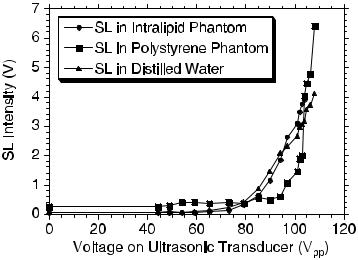
94 |
Optical Properties of Tissues with Strong (Multiple) Scattering |
a decrease in acoustic pressure in the negative half of a sinusoidal period; after the AW reaches the positive half of the period, the resulting pressure difference leads to a rapid collapse of the bubbles, accompanied by a broadband emission of light— SL. Such emission is of a short duration (in tens of picoseconds), repeatable with each cycle of sound, and has the spectrum containing molecular emission bands (with peaks near 300–500 nm) associated with the liquid, mostly water, in which the SL occurs.
SL tomography (SLT) as a new approach for optical imaging of dense turbid media (biological tissues) is described in Refs. 532 and 533. The major advantages of SLT include: (1) high SNR due to the internally generated probe optical signal;
(2) high contrast of imaging; (3) good spatial resolution, which is limited by the US focal size; and (4) low cost of equipment. It was shown experimentally that there is a threshold of SL generation at applied US pressure, when the peak pressure at the US focus was 2 bars ( 100 V, see Fig. 1.42). The rapid increase of the SL intensity with the acoustic pressure above the threshold indicates that the SL signal would be a sensitive measure of the local acoustic pressure. It is also seen in Fig. 1.42 that generation of SL is not affected by the addition of Intralipid and trypan blue, but is significantly affected by the addition of polystyrene spheres. Because SL is a broadband emission, the scattering and the absorption spectra of tissues and immersion liquids should be accounted for in imaging algorithms.533 On the basis of the calculated diffuse transmittance of the polystyrene phantom near 400 nm, the SL power at the source was estimated to be greater than 1 pW. The turbid media (tissue) functions as a filter that modifies the spectrum of the SL signal. For a cubic object made from rubber buried in the Intralipid phantom, the spatial resolution of the edges was estimated to be 2–3 mm, and an excellent imaging contrast was observed.533
Figure 1.42 SL intensity versus the driving voltage on the US transducer.533
Tissue Optics: Light Scattering Methods and Instruments for Medical Diagnosis |
95 |
SLT is based on several contrast mechanisms:533 (1) for the objects with US contrast relative to the background, the SL signal originating from the object differs from that originating from the background medium, the SL generation is affected by the local US intensity (see Fig. 1.42); (2) for the objects with contrast in optical properties, the SL signal from the object is attenuated differently because the SL light must propagate through the object; (3) for objects with the ability to generate SL, the SL from the object is different, even if the local US pressure is the same.
It should be noted that the peak pressure at the US focus is typically less than2 bars (1.3 W/cm2 in spatial-peak-temporal-peak power), which is one order in magnitude less than the safety limit set by the US FDA (23 bars) and two orders less than the tissue damage threshold (400 and 900 W/cm2 at 1 MHz for brain and muscle, respectively).533
1.5.9 Prospective applications and measuring techniques
It was recently shown that OA imaging allows one to perform highly resolved 3D images of artificial blood vessels in a tissue phantom with 20-μm depth resolution and 200-μm resolution in a lateral direction.477 The designed measuring technique and reconstruction algorithm were applied to image a vascular tree from a Wistar rat in vitro480 and human wrist skin blood vessels in vivo.481 In Ref. 481, a double-ring OA sensor together with measurements of a cross-correlation between the signals detected by the two rings were used to provide a narrow angular aperture of the system. The depth position of the observed vessels of the human wrist was about 1.5 to 2 mm below the skin surface. It was also demonstrated that besides skin and superficial blood vessels, the underlying bone was also identified, at a depth of about 3 mm below the skin surface.481 The total data acquisition time for getting a 2D image with 101 measurement positions (A-scans) was about 5 min for laser with a pulse repetition rate of 10 Hz. The maximum depth at which vessels can be detected is dependent on parameters such as the illuminating light intensity, the wavelength used, and the sensitivity of the OA sensor.
The feasibility of using the OA method for the monitoring of glaucoma treatment by application of a laser cyclophotocoagulation technique was proved recently.488 From described results it follows that the laser OA method seems to be a promising tool for localization of the ciliary body and monitoring of the coagulating process. In order to optimize fundus laser treatments of the eye, an online noninvasive OA technique for monitoring of fundus temperature was designed.489 It was found that the OA method can be used to noninvasively determine retinal temperatures during pulsed laser treatment of the eye. This technique can also be adapted to CW photocoagulation, photodynamic therapy and transpupillary thermotherapy, or other fields of laser-heated tissue.
Optoacoustics is used for the characterization of layered tissue structures in the near and far fields471 that is important to provide in-depth measurements of port wine stain of the human skin.474 The OA method can be also used to perform in vivo tomographic images of small animals. The 2D OA images475 as well as
96 |
Optical Properties of Tissues with Strong (Multiple) Scattering |
slices of a 3D image476 of sacrificed mice were reported. A system capable of performing OA structural and functional imaging in rat brain was developed.483,484
One more important application of the time-resolved OA technique is monitoring tissue mechanical response and ablation.511
Measurement of the pressure transient or displacement at the tissue surface is the most commonly provided by the use of piezoelectric sensors.458,459,481 Al-
though piezoelectric sensors have the advantage that broadband sensors are easy to construct and their sensitivity is rather high, optical methods may sometimes
be preferable in in vivo studies due to their ability to provide noncontact measurements (see Fig. 1.33).473,485–487 A minimally invasive noncontact interferometric
technique to accurately measure the effective optical attenuation depth of a sample is described.486,487 This technique measures the time-resolved tissue surface
displacement that results from absorption of a short laser pulse. The surface motion is caused by thermoelastic stress relaxation, whose time constant is proportional to the optical attenuation depth of the sample. The magnitude of expansion is a function of the incident radiant exposure and thermophysical properties of the sample. This technique is complementary to interferometric photothermal spectroscopy, a method that determines the effective optical attenuation depth through
time-resolved measurements of surface displacement resulting from the thermal diffusion that follows the thermoelastic stress relaxation process.509,510 The inter-
ferometric system utilizes a time-resolved high-resolution interferometer capable
of angstrom-level displacement resolution and nanosecond temporal resolution to detect subsurface blood vessels within a human forearm in vivo.486,487
High resolution and minimal artifacts of the images are characteristic for
the circular-scanning OA computed tomography with a full 360-deg scan about an object with elevated geometry, such as brain and breast.483,484,517,518 Planar reflection-mode techniques458,459,465,477 are not limited by the shape of the sample,
but they may suffer from the strong OA waves emitted from optical absorbers near the surface, such as hair follicles and melanin granules in the skin, whose acoustic reverberations can potentially overshadow the much weaker OA signals from structures deep in the tissue. A reflection-mode microscopic OA imaging technique that uses dark-field illumination prevents the occurrence of such artifacts.518 High image resolution and high sensitivity were achieved by utilizing a high-frequency, large-numerical-aperture (NA) spherically focused ultrasonic transducer that is coaxial and confocal with the optical illumination. Both a wide bandwidth and a large NA provide the high resolution of the acoustic detector; however, the increasing of frequency is limited because of a corresponding decrease of the acoustic wave penetration depth (attenuation in a tissue is of 0.7–3 dB/cm/MHz). Therefore, the OA sensor with a large NA (= 0.44) and frequency range from 32.5 to 67.5 MHz was used by the authors of Ref. 518 in in vitro and in vivo studies of rat skin. These parameters of the OA sensor provide lateral resolution of 45–120 μm (defined by the NA) and axial resolution of 15 μm (defined by the frequency range). The system is capable of imaging optical-absorption contrast as deep as 3 mm in tissue.
Tissue Optics: Light Scattering Methods and Instruments for Medical Diagnosis |
97 |
In monitoring and determining chemical traces, the time-resolved OA tech-
nique and other optothermal techniques may be prospective procedures to be used in noninvasive monitoring of glucose534–546 and blood hemoglobin volume and oxygenation.516,547,548
In the low-scattering mode when aqueous glucose solutions were irradiated by NIR laser pulses at wavelengths that corresponded to NIR absorption of glucose (1.0–1.8 μm), OA signal generation was assumed to be due to initial light absorption by the glucose molecules.536 A linear relationship between the OA signal and glucose concentration was found. It was also shown that the OA signal tracks change in glucose concentration in human measurements. No specific advantages of OA spectroscopy over an NIR measurement of glucose are expected in this case.534
Another approach of OA glucose detection is based on the glucose property to change scattering parameters of tissues.172,339–341,534,549–551 As follows from
Eq. (1.125), the OA signal from the tissue depth is defined by optical attenuation μeff, which is related to changes in the refractive index of the medium induced by changes in glucose concentration. Decreasing scattering increases the energy density in the OA sound source and induces higher OA signals.541 OA temporal profiles induced by 355-nm laser pulses in in vivo rabbit sclera at intravenous glucose administering demonstrated that a 1 mM increase in glucose concentration resulted in up to a 5% decrease of μeff.537 The UV light used in this experiment allowed one to increase the absolute value of the OA signal and its sensitivity to scattering change due to much higher absorption and scattering of tissues in UV than in the visible and NIR [see Eq. (1.125)].
However, in the NIR range, the effect of glucose on the scattering properties of tissue phantoms is also detectable by using the OA technique.540,541 At 905 nm,
a 1% (1 g dl−1) change in glucose concentration increased the OA signal by 2.0% in distilled water, 5.4% in 3% milk, and 2.5% in bloodless tissue, and at 1064 nm the similar change in glucose concentration increased the OA signal by 2.7% in 1% Intralipid. It was also found that the glucose-induced change in the OA signal was larger in blood than in Intralipid, amounting to 6.0%/0.5 g dl−1 of added glucose at 532 nm and 11.4%/0.5 g dl−1 of added glucose at 1064.540 Glucose-induced changes in the 1% Intralipid can be explained by a matching of refractive indices of phospholipid micelles and water with added glucose, whereas the observed
changes in blood may be additionally influenced by the changes in the size and shape of red blood cells due to changes of blood plasma osmolarity.48,538,540,552
Besides the increase in the peak-to-peak value of the OA signal as a function of glucose concentration, a corresponding shift in the position of the OA signal maxi-
mum toward earlier times at higher glucose concentrations, produced by changes in the sound velocity of the sample at glucose addition, was found.540,543 The other
two parameters in Eq. (1.125), the thermal expansion coefficient β and tissue or blood specific heat cT , also may be changed with a glucose concentration change. Estimations done in Ref. 541 showed that variations of these two parameters are not so high and do not seriously influence the OA signal in the limits of physiological glucose concentrations. As for the sound velocity dependence on glucose
98 |
Optical Properties of Tissues with Strong (Multiple) Scattering |
concentration, it may be excluded from the measurements of the OA temporal profile and give additional information on glucose concentration.
One of the drawbacks of the OA technique is that measurement of sound propagation in tissue is dependent on mechanical coupling between the tissue and the measuring probe and on the pressure of the probe on the tissue surface. This effect is quite similar to ultrasound propagation in tissue where coupling gels are used to decrease sound reflections.
Still further work is needed to understand OA signal origination and propagation in tissue and its use for glucose sensing. At present, the OA technique based on scattering measurements also does not offer any noticeable advantage over other scattering methods.534 However, a few groups and companies, such as Glucon, Inc.,542 are developing different new approaches for OA glucose sensing, including techniques based on combining ultrasound and OA spectroscopy.534
Thermal gradient spectroscopy (TGS) is based on measuring the fundamental
absorption bands of glucose at 9.1–10.5 μm using the body’s naturally emitted IR radiation as an internal source of radiation.534,544–546 The cooling-induced skin
transparency allows for monitoring of IR emission from the interstitial fluid and cutaneous layers.544,545 A linear response between in vivo TGS detected glucose
and reference blood glucose values has been reported in clinical studies for several individuals with Type 1 diabetes.544 Different modifications of this method and
corresponding instrumentation for more precise quantifying of glucose in a human body are described in the literature.534,545,546 The simplicity of this method makes
it quite appealing; however, the overlap between the effect of glucose on the signal and temperature variations due to circadian periodicity, as well as temperature and blood flow response to glucose change, should be eliminated or accounted for.534 An OA laser system for noninvasive monitoring of cerebral venous oxygenation in the superior sagittal sinus based on a Q-switched nanosecond Nd:YAG laser (wavelength 1064 nm, pulse repetition rate 1 Hz) was designed.516 The authors demonstrated that the amplitude and temporal profile of OA waves are linearly dependent on blood oxygenation in the wide range of blood oxygenation from 24% to 92%. The designed system was capable of real-time and continuous measurements of blood oxygenation despite optical and acoustic attenuation by thick bone.
The use of an OA technique for noninvasive and real-time continuous monitoring of total hemoglobin concentration (THb) was recently proposed.547,548 It was
shown that the OA technique may provide accurate measurements of THb by detection and analysis of OA signal temporal profiles induced by short optical pulses in blood circulating in arteries or veins. A portable OA system based on a 10-ns Nd:YAG laser (1064 nm) was designed for the monitoring of THb in the radial artery. Results of in vitro and in vivo studies demonstrated that (1) the slope of OA waves induced in blood in the transmission mode is linearly dependent on THb in the range from 6.2 to 12.4 g/dl; (2) OA signals can be detected despite optical attenuation in turbid tissue phantoms with a thickness of 1 cm; and (3) the OA system detects signals induced in blood circulating in the radial artery. Clinical studies for healthy volunteers, described in Ref. 548, showed that the amplitude of
Tissue Optics: Light Scattering Methods and Instruments for Medical Diagnosis |
99 |
OA signal generated in the radial artery closely followed the THb (rapidly changed at infusion of intravenous saline) measured directly in concurrently collected blood samples.
The photothermal microscopy (PTM) technique shows the capability to visualize absorbing cellular structures of living cells in vitro without labeling,503–506
as well as to image moving unlabeled cells in real time in vivo in studies of cir-
culating red and white blood cells in capillaries and lymph microvessels of rat mesentery.507,508 We will briefly discuss some potential applications of this optical
tool called PT flow cytometry (PTFC).508 The imaging of single cells in vivo is potentially important for the early diagnosis of diseases (e.g., cancer and diabetes) or for the study of the influence of various factors (e.g., drugs, smoking, ionizing radiation) on individual cells.
To realize PTFC, a nonscanning fast PTM system was used because of cells crossing the area of detection in 0.1–0.01 s for even relatively slow flow in capillaries.508 Such a system was built on the basis of a pulsed pumping tunable optical parametric oscillator (420–570 nm, pulse width of 8 ns, pulse energy of 0.1–400 μJ; Lotis Ltd.). Laser-induced temperature-dependent variations of the refractive index in the cell were detected using a phase-contrast imaging technique (Olympus BX51 microscope with a CCD camera; AE-260E, Apogee Inc.) with illumination by a low-energy collinear probe pulse (Raman shifter, wavelength 639 nm, pulse width of 13 ns, and pulse energy of 2 nJ). The diameters of the pumpand probe-beam spots, with stable, smooth intensity profiles, ranged from 20 to 50 μm and 15 to 50 μm, respectively, and thus covered entire single cells and even whole microvessels. A spatial resolution of 0.7 μm was provided. The acquisition procedure included illumination of the cell with three pulses: an initial probe pulse followed by a 0.08-s delay to the pump pulse, and then a second probe pulse with a tunable time delay (0–5000 ns) to the pump pulse. The PT image, calculated as the difference between the two probe-pulse images, depends only on absorption contrast transformed by the pump laser pulse into refractive contrast.508
To experimentally prove the concept of in vivo PTFC, a rat mesentery model was chosen among various animal models (e.g., ears, lips, etc.) because of its unique anatomic structure consisting of thin, transparent, duplex connective tissue with a single layer of blood and lymph microvessels. Using transillumination digital microscopy (TDM) RBCs and lymphocytes traveling through blood and/or lymph vessels, lymphatic valves, and other mesenteric structures were imaged (Fig. 1.43). It was found that in most intact lymph vessels (diameter of 50– 150 μm), lymphocytes in flow had an average velocity of 211 ± 11 μm/s. In comparison, the velocity of RBCs was significantly higher, up to 2 mm/s in blood vessels with a diameter of 20–30 μm and from 100 to 500 μm/s for capillaries with diameter less than 10 μm. The high spatial resolution of TDM (300 nm at 100×, NA = 1.25 with immersion) allowed roughly estimating the cell size and even shape (Fig. 1.44, left). Because of its low absorption sensitivity, however, TDM was not suitable for visualizing absorbing cellular structures. In contrast, the PTFC mode (navigated by TDM) allowed the obtaining of images of moving lymphocytes and RBCs (Fig. 1.44, right) that showed structures specific to PT images and

100 |
Optical Properties of Tissues with Strong (Multiple) Scattering |
Figure 1.43 Typical optical image of a lymph microvessel of rat mesentery with blood microvessels along the lymphatic walls (bottom), RBCs in a capillary (top left), and single cells in lymph flow (top right).508
associated with the spatial distribution of absorbing cellular chromophores (e.g., hemoglobin in RBCs, or cytochromes in lymphocytes). Currently, PTFC’s rate of10 cells/s is limited by the repetition rate of the pump laser (10 Hz).
Potential applications of in vivo PTFC may include: (1) identification of cells with differences in natural absorptive properties (e.g., the counting of white cells in blood flow or of rare RBCs among lymphocytes in microlymphatic vessels); (2) monitoring of the circulation and distribution of absorbing nanoparticles used for PT probing or photosensitizing; (3) study of laser-cell interactions; and
(4) study of the influence of different environmental factors on cells.
The main technical difficulty of the time-resolved measurements of OA profiles is associated with correct detection of acoustic signals, which requires simultaneously high temporal resolution equal to or higher than the laser pulse duration and wideband frequency detection extending into low-frequency ultrasound.458 Wideband piezoelectric transducers with short-circuit or open-circuit operating modes, being low-noise detectors, have proved to be most suitable for this purpose. The transducer operating in the short-circuit mode has substantial thickness that is larger than the spatial width of the detected ultrasonic transient. The transducer thickness limits the lower limit of detected ultrasonic frequencies and duration of the detection window. An excessively thick piezoelement would: (1) lead to a more prominent acoustic diffraction at lower ultrasonic frequencies in the detected signal, and (2) reduce the electric capacity to a value below the electric capacity of the electronic circuitry. It is difficult to design acoustic transducers operating in short-circuit mode for detection of OA profiles longer than 1–2 μs. However, these

Tissue Optics: Light Scattering Methods and Instruments for Medical Diagnosis |
101 |
Figure 1.44 Optical transmission (left column) and PT (right column) images in vivo of a single, moving lymphocyte (top row) and RBCs (bottom row) in lymph flow in rat mesentery (vessel diameter 105 μm, velocity 120 μm/s). Pump pulse parameters: wavelength, 525 nm; pulse width, 8 ns; and pulse energy, 30 μJ and 0.5 μJ (right column, top and bottom, respectively); time delay between pump and probe pulses, 10 ns.508
transducers would be most optimal for detection of submicrosecond and nanosecond OA signals. The upper limit of ultrasonic frequency is defined by the discharge time of the transducer capacity. The ultrasonic detection band could reach several hundred megahertz. This type of transducer does not require backing material to reduce resonant vibrations.
In the case of an acoustic transducer operating in the open-circuit mode, it is necessary that the thickness of piezoelectric element be smaller than the acoustic wavelength detected in its upper ultrasonic frequency limit.458 The lower limit of detectable ultrasonic frequencies is defined by the discharge time of the transducer electric capacity through the input resistor of the electronic preamplifier. In order to design acoustic transducers operating in the open-circuit mode with very wide ultrasonic detection band (≥100 MHz), one has to employ piezoelectric elements that are a few microns thick. The choice of appropriate backing material is crucial for widening the frequency band. Design of the backing layer acoustically matched with the piezoelectric material for effective damping of transducer resonances is one of the most important technical problems. The sensitivity of open-circuit transducers is greater than that of short-circuit transducers due to longer holding of the electric charge at the piezoelement.
Another technical difficulty in providing high temporal resolution in the detection of OA profiles is the need for precise adjustment of the detector face with respect to the wavefront of the arriving optoacoustic signal.458 Obviously, the time difference between the instances of the laser-induced pressure transient (LIPT) ar-
102 |
Optical Properties of Tissues with Strong (Multiple) Scattering |
rival to the opposite edges of the piezoelectric element should be shorter than the temporal resolution of this transducer. Therefore, the angle between the direction of the LIPT wavefront propagation and the normal to the piezoelectric detector must be as small as possible. For example, to achieve temporal resolution of τ10 ns, the LIPT has to be incident with angle by less than 3 min relative to the sensitive area aperture of 3 mm.
The highest possible piezoelectric efficiency for wideband piezoelectric detection can be achieved with piezoceramics, such as PZT-5H.458 A lower sensitivity could be obtained with polyvinyldenefluoride (PVDF) or PVDF copolymers. Quartz and lithium niobate have significantly lower sensitivity for wideband ultrasonic detection.
Low acoustic impedance, which is similar to that in biological tissues, makes PVDF suitable for applications in medical and biological sensing.458 Design of effective backing for PVDF transducers does not represent a great problem and makes detected OA signals clear from reverberations within the piezoelement.
There are a number of designs of wideband acoustic and OA transduc-
ers that may be employed for a variety of applications in biomedicine (see Fig. 1.35).458,467,518 Two-dimensional OA images can be provided either by using a
stationary array of acoustic transducers or by scanning a single transducer along the tissue surface.459 The arc-shaped array containing 32 ultrawideband piezoelectric transducers with 1× 12.5-mm size and a distance of 3.85 mm between the elements is described.459 The 110-μm-thick piezoelectric polymer PVDF was used to provide an ability to operate in a wide ultrasonic frequency band. The transducers were mounted on the arc surface with a radius of 60 mm; thus, such geometry provided optimal resolution in the entire 60 × 60-mm field of view within the image plane. The shape and length of individual piezoelements determine spatial resolution of this array in the plane perpendicular to the image plane. The flat elements used provided a resolution equal to the linear size of the element. This 32-element array was used for the acquiring of two-dimensional OA images of breast tumors.459 Two images at two different laser wavelengths of 1064 and 757 nm were acquired in succession at irradiation with sixteen 100-ns pulses at each wavelength over the course of 0.8 s. Image reconstruction took about 1 s. Resolution of the image visualization was 1 mm along the depth axis and 1.5 mm in the lateral direction, which is comparable to that of x-ray mammography and ultrasound.
Three-dimensional OA imaging can be provided using the system designed by LaserSonix Technologies, Inc. which is based on a bifocal array of 64 piezoelectric transducers and corresponding 64 data acquisition channels.459 This system has close-to-real-time image acquisition and data processing with a resolution of about 3 mm in the plane perpendicular to the image plane, so that thin frontal slices of the breast can be visualized. Full-field-of-view 3D images can be reconstructed by fusing sixty 2D slices. A fast OA imaging system based on a 320-transducer linear array was also recently developed and tested.553
A high-resolution confocal OA transducer that provides subsurface imaging in the scanning mode is applicable when a superhigh resolution on the cellular or
Tissue Optics: Light Scattering Methods and Instruments for Medical Diagnosis |
103 |
subcellular level is needed.459 An ultrawide band of ultrasonic detection realized in front-surface transducers yields an in-depth resolution close to 15 μm. In incident optical beam focusing, a comparable lateral resolution is also achievable. The confocal OA transducer provides sharp focusing of the optical beam and a long narrow waist of acoustic focus in the ultrasonic detection system. The distributions of focused light and the caustic of the ultrasonic detection define the measuring volume of the confocal transducer.
Another modification of an OA sensor used in the dark-field reflection-mode imaging system, containing an optical fiber that is coaxially positioned with a focused ultrasonic transducer and attached to a concave lens, is described in Ref. 518. A variety of OA probes suitable or already tested for OA spectroscopy and imaging of biological tissues and blood are described in Refs. 512, 515, 516, 540, 541, 547, 548, and 553–557.
1.5.10 Conclusion
OTR, OA, and PA transient techniques provide a convenient means for in vitro, or even in vivo and in situ, monitoring of optical and thermal properties of a variety of human tissues, including skin. In particular, water content and surface concen-
tration and diffusion of topically applied substances (drugs and sunscreens) can be measured.460,490–492 The main difficulty of the PA method in the case of in vivo
measurements is the requirement for a closed sample cell that can efficiently guide the acoustic signal from sample to microphone.
The use of pulsed OA and OTR techniques is more appropriate for in vivo and in situ experiments. The optothermal and optothermoelastic responses of a living tissue on pulse laser excitation discussed are the basis for a novel approach in med-
ical tomography that combines achievements of optical, thermal, and acoustical probing of a tissue.458,459,517
A variety of tissue imaging techniques are suggested on the basis of US and light beams interacting within an inhomogeneous medium that occurs through
the change in optical properties of the medium resulting from its compression by the US.517,519–542 These are so-called acousto optical (AO) interactions and imag-
ing technologies.
To OA and AO signals contribute any scattered photons (singly and multiply); therefore, the imaging depth is extended compared with other ballistic or quasiballistic imaging modalities, such as OCT or confocal microscopy.
The OA and AO tomographies (OAT and AOT) provide:517 (1) a combination of high optical contrast and high acoustic resolution; (2) a potential for simultaneous functional imaging of blood oxygenation and blood volume; (3) a high ratio between imaging depth and resolution; (4) no speckle artifacts; (5) scalable resolution and imaging depth by varying the US frequency; (6) an ability to simultaneously acquire OAT/AOT images and pure US images from the same cross sections of the sample for added diagnostic value; and (7) nonionizing laser and US radiation within the safety limits for biological tissues.
104 |
Optical Properties of Tissues with Strong (Multiple) Scattering |
However, OAT and AOT have some limitations mostly associated with the usage of US technology. They are: contact measurements, which are required for acoustic coupling, and strong US wavefront aberrations induced by some heterogeneous tissues and organs. In the case when acoustic heterogeneity is strong, concurrent US imaging may be useful for providing the acoustic properties that are needed for image reconstruction in OAT or AOT.
1.6 Discrete particle model of tissue
1.6.1 Introduction
Although it follows from the preceding discussion that the optical properties of tissue are related to its microstructure and refractive index distribution, the nature of the relationship should be discussed in more detail. It has been shown that the contribution of mitochondria and spatial variations in the refractive index of cells and
other tissue components, such as collagen and elastin fibers, to the scattering properties of tissue can be estimated theoretically and experimentally.58,85,96,154,156,558
However, the quantitative model that relates the microscopic properties of cells and other tissue components to the scattering coefficients of bulk tissue is still not completed. Ideally, such a model should be able to predict the absolute magnitudes of the optical scattering coefficients as well as their wavelengths and angle dependencies.156 The model should provide insight into how the scattering properties are influenced by the numbers, sizes, and arrangement of the tissue components in order to be useful for inverse problem solving. This section presents a framework for a particulate model of soft tissue that satisfies at least a few of these requirements. The model was developed by the authors of Ref. 156; their paper is discussed.
1.6.2 Refractive-index variations of tissue
Soft tissue is composed of closely packed groups of cells entrapped in a network of fibers through which water percolates. At a microscopic scale, the tissue components have no pronounced boundaries. They appear to merge into a continuous structure with spatial variations in the refractive index. To model such a complicated structure as a collection of particles, it is necessary to resort to a statistical approach.
It has been shown that the tissue components that contribute most to the local refractive-index variations are the connective tissue fibers (bundles of elastin
and collagen), cytoplasmic organelles (mitochondria, lysosoms, and peroxisomes), cell nuclei, and melanin granules.58,154,156 Figure 1.45 shows a hypothetical index
profile formed by measuring the refractive index along a line in an arbitrary direction through a volume of tissue. The widths of the peaks in the index profile are proportional to the diameters of the elements, and their heights depend on the refractive index of each element relative to that of its surroundings. In accordance

Tissue Optics: Light Scattering Methods and Instruments for Medical Diagnosis |
105 |
with this model, the origin of the index variations will be presented by a statistically equivalent volume of discrete particles having the same index but different sizes.
The refractive indices of tissue structure elements, such as the fibrils, the interstitial medium, nuclei, cytoplasm, organelles, and the tissue itself, can be derived using the law of Gladstone and Dale, which states that the resulting value repre-
sents an average of the refractive indices of the components related to their volume fractions as442
N
$$
n¯ = ni fi , |
fi = 1, |
(1.150) |
i=1 |
i |
|
where ni and fi are the refractive index and volume fraction of the individual components, respectively, and N is the number of components.
Figure 1.45 Spatial variations of the refractive index of a soft tissue. A hypothetical index profile through several tissue components is shown, along with the profile through a statistically equivalent volume of homogeneous particles. The indices of refraction labeling of the profile are defined in the text.156
The statistical mean index profile in Fig. 1.45 illustrates the nature of the approximation implied by this model. The average background index is defined as the weighted average of the refractive indices of the cytoplasm and the interstitial fluid, ncp and nis, as
n¯ 0 = fcpncp + (1 − fcp)nis, |
(1.151) |
where fcp is the volume fraction of the fluid in the tissue contained inside the cells. Literature data presented in Ref. 58 allow one to estimate ncp = 1.367 and nis = 1.355. Since approximately 60% of the total fluid in soft tissue is contained in the intracellular compartment, it follows from Eq. (1.151) that n¯ 0 = 0.6(1.367) + 0.4(1.355) = 1.362. The refractive index of a particle can be defined as the sum of the background index and the mean index variation,
n¯ s = n¯ 0 + n , |
(1.152) |
106 |
Optical Properties of Tissues with Strong (Multiple) Scattering |
|
which can be approximated by another volume-weighted average, |
|
|
|
n = ff(nf − nis) + fnc(nnc − ncp) + for(nor − ncp). |
(1.153) |
Here, the subscripts f, is, nc, cp, and or refer to the fibers, interstitial fluid, nuclei, cytoplasm, and organelles, respectively, which were identified above as the major contributors to index variations. The terms in parentheses in this expression are the differences between the refractive indices of the three types of tissue component and their respective backgrounds; the multiplying factors are the volume fractions of the elements in the solid portion of the tissue. The refractive index of the connective-tissue fibers is about 1.47 (see Table 2.2), which corresponds to about 55% hydration of collagen, its main component. The nucleus and the cytoplasmic organelles in mammalian cells that contain similar concentrations of proteins and nucleic acids, such as mitochondria and the ribosomes, have refractive indices that lie within a relative narrow range (1.38–1.41).58 Taking this into account and assuming that nnc = nor = 1.40, the mean index variation can be expressed in terms of only the fibrous-tissue fraction cf as
n = ff(nf − nis) + (1 − ff)(nnc − ncp). |
(1.154) |
Collagen and elastin fibers compose approximately 70% of the fat-free dry weight of dermis, 45% of the heart, and 2–3% of nonmuscular internal organs (see Refs. 14–16 in Ref. 156). Therefore, depending on tissue type, ff may be as small as about 0.02 or as large as 0.7. For nf − nis = 1.470 − 1.355 = 0.115 and nnc − ncp = nor − ncp = 1.400 − 1.367 = 0.033, the mean index variations that correspond to these two extremes are n = 0.02(0.115) + (1 − 0.02)(0.033) = 0.035 and n = 0.7(0.115) + (1 − 0.7)(0.033) = 0.09.
1.6.3 Particle size distributions
For some tissues, the size distribution of the scattering particles may be essentially monodispersive and for others it may be quite broad. Two opposite examples are transparent eye cornea stroma, which has a sharply monodispersive distribution, and turbid eye sclera, which has a rather broad distribution of collagen fiber diameters.129 There is no universal distribution size function that describes all tissues with equal adequacy. In the optics of dispersed systems, Gaussian, gamma, or power size distributions are typical.171 Polydispersion for randomly distributed scatterers can be accounted for by using the gamma distribution or
the skewed logarithmic distribution of scatterers’ diameters, cross sections, or volumes.61,129,154,156,165,172 In particular, for turbid tissues such as eye sclera, the
following gamma radii distribution function is applicable:61,172
η(a) = aμ exp(−μβ), |
(1.155) |
Tissue Optics: Light Scattering Methods and Instruments for Medical Diagnosis |
107 |
where σ/am = 2.35μ−0.5, β = a/am, σ is the half-width of the distribution, and am is the more probable scatterer radius.
A two-phase system made up of an ensemble of equally sized small particles, and a minor fraction of larger ones, provides a good model of pathological tissue, e.g., a cataractous lens.173
For epithelial cells and their nuclei scattering structures, log-normal size distributions of spherical or slightly prolated ellipsoidal particles are characteristic
as166 |
|
aσ√2π |
− [ |
|
|
|
|||
|
= |
2σ2 |
|
||||||
η(a) |
|
1 |
|
exp |
|
ln(a) − ln(am)]2 |
. |
(1.156) |
|
|
|
|
|
|
|
||||
In particular, for epithelial cells and their nucleus components, two log-normal size distributions for small and big spherical scatterers with the following parameters were found in a certain line of rat prostate carcinoma cells:166 am1 = 0.012 μm, σ1 = 1.15 μm, and am2 = 0.59 μm, σ2 = 0.43 μm.
For the description of scattering characteristics of a particle with a complex
shape, different from a sphere or long cylinder, some special procedures, for example, the method of T-matrices, can be applied.145,146,166 Complexly shaped scatter-
ers, like cells themselves, may be modeled as aggregates of spherical particles. The scattering centers in turbid tissue have a wide range of dimensions and
tend to aggregate into complex forms suggestive of fractal objects. The skewed logarithmic distribution function is used extensively in particle-size analysis as being the most plausible on physical grounds. The skewed logarithmic distribution function for the volume fraction of particles of diameter 2a is156
|
= |
Cm |
|
|
|
− |
|
|
− [ |
|
|
2σ2 |
|
|
|
|
|
η(2a) |
|
Fv |
(2a)3 |
|
Df exp |
|
|
ln(2a) |
− ln(2am)]2 |
, |
(1.157) |
||||||
|
|
|
|
|
|
|
|
||||||||||
where |
|
|
|
|
|
|
|
|
|
|
|
|
|
|
|
|
|
|
|
|
|
|
|
|
|
|
|
|
|
|
D |
2σ2 |
|
|
|
Cm = σ√2π(2am)4−Df exp |
|
|
|
|
|||||||||||||
(4 − f ) |
|
|
|
|
|||||||||||||
2 |
|
|
|
||||||||||||||
is the normalizing factor; |
|
|
|
|
|
|
|
|
|
|
|
|
|
|
|
||
|
|
|
|
Fv = 0 |
∞ η(2a)d(2a) |
|
|
|
|
|
|||||||
is the total volume fraction of the particles, and the quantities 2am and σ set the center and width of the distribution, respectively; Df is the (volumetric) fractal dimension.
In the limit of an infinitely broad distribution of particle sizes,
η(2a) ≈ (2a)3−Df . |
(1.158) |
108 |
Optical Properties of Tissues with Strong (Multiple) Scattering |
For 3 < Df < 4, this power-law relationship describes the dependence of the volume fractions of the subunits of an ideal mass fractal on their diameter, 2a. These size distributions expand the size distributions described by Eqs. (1.155) and (1.156) to account for the fractal properties of tissues.
Scatterers in the epidermal layer of the skin also exhibit a log-normal size dis-
tribution, whereas the spatial fluctuations in the index of refraction of dense fibrous tissues, such as the dermis, and many other tissues follow a power law.107,165
1.6.4 Spatial ordering of particles
A discrete particle ensemble is characterized by the packing density or, in other words, by the volume fraction occupied by particles. Evidently, in addition to particle size, the volume fraction of particles is also essential for the optical properties of an ensemble due to its influence on the refractive index distribution [see Eqs. (1.150)–(1.154)], optical anisotropy [see Eqs. (1.53) and (1.54)], and other structure characteristics. The volume fraction of particles for a certain tissue may be experimentally found using electron micrographs of tissue slices. Estimations of a volume fraction occupied by scattering particles may also be accomplished by the weighting of a native tissue and dry rest.
The volume fraction occupied by the scattering particles in tissues, such as muscle, cornea, sclera, and eye lens, covers from 20 to 40%. Conventionally, whole blood contains (4–5) × 106 erythrocytes, (4–9) × 103 leukocytes, and (2–3) × 105 platelets in 1 mm3. Cells make up 35–45% of the blood volume. The volume fraction f of erythrocytes in the blood is called the hematocrit H . For normal blood, H = 0.4. The remaining 60% of the blood volume is mostly the plasma—an essentially transparent water solution of salts.
Most tissues are comprised of cellular and subcellular structures located in close proximity to each other. In general, densely packed structures are likely to
exhibit correlation scattering, an effect that has been observed, for instance, in corneal stroma.63,129,432,433,435,436 Cornea is comprised of individual collagen fib-
rils that are closely packed and parallel to one another in a lamella. If each fibril in the lamella scattered light independently, then the scattering cross section of the lamella should be the product of the cross section of a single fibril and the number of fibrils in the lamella. If all of the cornea fibers scattered light independently, the cornea would scatter 90% of the light incident on it, and we would see essentially nothing. However, the fibrils do not scatter independently and the coherent scatter-
ing (interference) effects cannot be neglected. Accordingly, correlated polarization effects can be observed.63,435–438 For example, in spherical particle suspensions,
as the particle concentration increases beyond a concentration at which independent scattering can be assumed, the degree of polarization increases (rather than decreases) as the scatterer concentration increases.437,438
Thus, the spatial organization of the particles forming a tissue plays a substantial role in the propagation of light. As mentioned above, with very small packing densities, incoherent scattering by independent particles occurs. If the volume
Tissue Optics: Light Scattering Methods and Instruments for Medical Diagnosis |
109 |
fraction occupied by the particles is equal to or more than 0.01–0.1, coherent concentration effects appear. The concentration of scattering particles is adequate in most tissues to allow spaces between individual scatterers that are comparable to their sizes. If, however, the particle-size distribution is rather narrow, then dense
packing entails a certain degree of order in the arrangement of the particles. Spatial ordering is of utmost importance in optical eye tissue.63,64,129,403,432,
433,435,436 In a large variety of other tissues, spatial ordering is also more or less inherent, particularly in tendon, cartilage, dura mater, skin, or muscle. The high degree of order in densely packed scatterers ensures high transmission in the cornea and eye lens. Tissue structures with statistically ordered periodical variations in the index at characteristic scales of light wavelength, like photonic crystals,440 exhibit high-transmission spectral regions and bands for which the propagation of electromagnetic waves is forbidden. The position and depth of these bands depend on the size, refractive index, and spatial arrangement of the scattering particles.
To account for the interparticle correlation effects, which are important for systems with volume fractions of scatterers higher than 1–10% (dependent on particle dimensions), the following expression for the packing factor of a medium filled with a volume fraction fs of scatterers with different shapes is valid:148
ω |
p = |
(1 − fs )p+1 |
, |
(1.159) |
|
[1 + fs (p − 1)]p−1 |
|||||
|
|
|
where p is a packing dimension that describes the rate at which the empty space between scatterers diminishes as the total density number increases. The packing of spherical particles is described well by packing dimension p = 3. The packing of sheetlike and rod-shaped particles is characterized by dimensions that approach 1 and 2, respectively. The elements of tissue have all of these different shapes and may exhibit cylindrical and spherical symmetry simultaneously, and the packing dimension may lie anywhere between 1 and 5. When one calculates the optical coefficients at high concentrations of particles, the size distribution η(2a)
[Eqs. (1.155)–(1.158)] should be replaced by the correlation-corrected distribution156
η (2a) |
= |
|
[1 − η(2a)]p+1 |
η(2a). |
(1.160) |
|
[1 + η(2a)(p − 1)]p−1 |
||||||
|
|
|
||||
Most of the observed scattering properties of soft tissue that are explained in the model treat tissue as a collection of scattering particles whose volume fractions are distributed according to a skewed log-normal distribution modified by a packing factor, to account for correlated scattering among densely packed particles.156
110 Optical Properties of Tissues with Strong (Multiple) Scattering
1.6.5 Scattering by densely packed particle systems
The spatial correlation of individual scatterers results in a necessity to consider the interference of multiply scattered waves. The particle reradiation in the densely packed disperse system induces the distinction of an effective optical field in a medium from the incident one. Under these conditions, the statistical theory of multiple wave scattering seems to be most promising for describing
the collective interaction between an ensemble of particles and electromagnetic radiation.75,442,559
The rigorous theory of wave multiple scattering is constructed on the basis of fundamental differential equations for the fields followed by using statistical
considerations. |
75 |
The total field |
at the point is the sum of the incident field |
|||||
|
|
|
|
|
E(r) |
|
r |
|
i (r) and the scattered fields from all particles with regard to their phases, |
|
|||||||
E |
|
|
|
|
|
|
|
|
|
|
|
|
= i + |
N |
j |
|
|
|
|
|
|
$ |
|
|||
|
|
|
|
E(r) |
E (r) |
Es (r), |
(1.161) |
|
|
|
|
|
|
||||
|
|
|
|
|
|
j =1 |
|
|
|
Es |
|
|
|
|
|
|
|
where j |
(r) is the scattered field of the j th particle. The field scattered by the |
|||||||
j th particle is defined by the parameters of this particle and by the effective field incident on the particle.
Twersky has derived a closed system of integral equations describing the processes of multiple scattering.560 A rigorous solution in a general form has not yet been found for this problem. In actual calculations, various approximations are exploited in order to perform the averaging of Eq. (1.161) over statistical particle configurations. For example, the quasi-crystalline approximation proposed for densely packed media by Lax561 is used most efficiently in tissue optics.442
Averaging of Eq. (1.161) over statistical particle configurations results in an infinite set of equations that is truncated at the second step by applying the quasicrystalline approximation. The closed system of equations obtained for the effective field is reduced to a system of linear equations by expansion in terms of vector spherical or cylindrical harmonics. The explicit expressions562,563 for the expansion coefficients involve the radial distribution function as well as the Mie coefficients for a single particle. The equality to zero for the determinant of this system of linear equations yields the dispersion relation for the effective propagation constant keff of this medium.564 For the systems of particles whose sizes are small
compared with the wavelength, the expression for keff obtained in this way has the
form442,562
keff2 = k2 + |
3fy |
k2 |
1 + i |
2 k2a2y |
S3(θ = 0) , |
(1.162) |
||
|
|
|
|
|||||
D |
3 D |
|||||||
Tissue Optics: Light Scattering Methods and Instruments for Medical Diagnosis |
111 |
where |
|
|
|
|
|
|
|
|
|
|
|
|
|
|
|
|
|||
y |
|
n12 − n02 |
, D 1 fy, S (θ 0) |
|
1 |
, H |
|
|
24f |
|
α β δ |
, |
|||||||
|
|
|
|
|
|
|
|
|
|
|
|
|
|||||||
|
|
|
|
3 |
|
3 + 4 + 6 |
|||||||||||||
|
= n12 + 2n02 = − |
3 |
= = 1 |
− H3 |
|
= − |
|
|
|||||||||||
|
|
|
|
|
|
||||||||||||||
|
|
|
|
|
|
|
|
|
|
|
|
(1.163) |
|||||||
in which f is the volume fraction occupied by particles with the radius a and the refractive index n1, and the α, β, and δ values are found according the approximation of hard spheres
α |
|
|
(1 + 2f )2 |
, |
β |
6f |
(1 + 0.5f )2 |
, δ |
|
1 |
f |
(1 + 2f )2 |
. |
(1.164) |
||||||
|
|
|
|
|
||||||||||||||||
|
= |
(1 |
− |
f )4 |
|
= − |
(1 |
− |
f )4 |
|
= 2 |
|
(1 |
− |
f )4 |
|
||||
|
|
|
|
|
|
|
|
|||||||||||||
The calculated effective index of refraction442 |
|
|
|
|
|
|
|
|
|
|||||||||||
|
|
|
|
|
|
|
|
neff = neff + ineff |
|
|
|
|
|
|
|
(1.165) |
||||
is complex, even if the particles and a base substance surrounding them exhibit no intrinsic absorption. The imaginary part of the effective index of refraction neff describes the energy diminishing for an incident plane wave due to scattering in all directions. The transmittance of this layer with thickness z is
T |
= |
exp |
− |
4π |
n |
z . |
(1.166) |
|
λ |
||||||||
|
|
eff |
|
|
The quantity μt = 4π neff/λ is the extinction coefficient. The value of the imaginary part of the effective index of refraction grows for these systems with a higher
radiation frequency and it nonmonotonously depends on the particle concentration in the layer. As a result, the transmittance of the disperse layer decreases for small particle concentrations with a greater concentration of particles and, starting at f ≈ 0.1, the transmittance grows and the so-called clearing effect takes place. The real portion of the effective index of refraction in this approximation is essentially independent of the wavelength and alters monotonously with growing particle concentration to approach the refractive index of the particles. The near ordering in the scatterers’ arrangement with their greater concentration not only provides for conditions for the manifestation of the secondary scattered wave interference, but it also changes the regime of propagation of noncoherent multiply scattered light.565 This may be accompanied by the so-called concentration effects of clearing and darkening.
The optical softness of tissues enables one to employ under calculation an expansion by scattering multiplicities with restriction by low orders. In Ref. 566, an expression was obtained for the effective index of refraction of the eye cornea modeled by the system of cylinder scatterers in the form of expansion by the scattering multiplicities, and the effects of polarization anisotropy were analyzed with respect to the double scattering contributions.

112 |
Optical Properties of Tissues with Strong (Multiple) Scattering |
Using the theory of multiple scattering, Twersky567 succeeded in deriving the approximate expressions for the absorption μa and scattering μs coefficients that describe the light propagation in the blood. The blood hematocrit Hct is related
to the erythrocyte concentration ρ and to the volume of an erythrocyte Ve by the following ratio:183,567
ρ = Hct/Ve. |
(1.167) |
Thus, the absorption factor μa is
μa = |
Ve |
σa. |
(1.168) |
|
|
|
Hct |
|
|
For sufficiently small values of Hct (Hct < 0.2), the scattering coefficient is given by the equation
μs = |
Ve |
σs. |
(1.169) |
|
|
|
Hct |
|
|
For Hct > 0.5, the particles become densely packed and the medium is almost homogeneous. In this case, the blood may be considered as a homogeneous medium containing hemoglobin in which scattering particles formed by plasma surrounding red blood cells are embedded. Within the limits of Hct → 1, “plasma particles”
disappear and the scattering coefficient should tend to zero. This results in the following approximate equation for μs:183,568
μ |
Hct(1 − Hct) |
σ |
, |
(1.170) |
|
||||
s ≈ |
Ve |
s |
|
|
where the coefficient (1 − Hct) regards the scattering termination with Hct → 1. However, the absolute dense packing (Hct = 1) is not attainable in reality; for example, for the hard sphere approximation, Hct may not exceed 0.64. Considering this fact and keeping in mind the physiological conditions, the affect of cell packing on light scattering might be described by a more complex function as
Hct |
σsF (Hct), |
|
μs = Ve |
(1.171) |
where the packing function F (Hct) accounts for physiological conditions of red
blood cells, in particular, cell deformability at high concentration.
Although the equations from Twersky’s wave-scattering theory560,567 agree reasonably well with measured optical density data for a whole blood layer,568 researchers have had to resort to curve-fitting techniques to evaluate the parameters in Twersky’s equations. This theory also does not describe the spatial distribution of the reflected and transmitted light, and therefore does not accommodate light

Tissue Optics: Light Scattering Methods and Instruments for Medical Diagnosis |
113 |
detectors and sources that do not share a common optical axis. By contrast, the radiative transfer theory discussed above—in particular, its more simple diffusion approximation—overcome listed limitations of the wave-scattering theory; but to be applied to densely packed tissues, this theory should account for particle interaction and size distribution effects. The combination with other theories describing particle interactions and the usage of empirical data can be considered as a fruitful and practical approach for modeling of the optical properties of tissues.
For example, using the diffusion theory, Steinke and Shepherd568 have corrected the dependence [Eq. (1.170)] of the scattering coefficient μs for a thin blood layer on the hematocrit Hct, as the following:
μs ≈ |
Ve |
σs(1 − Hct)(1.4 − Hct). |
(1.172) |
|
|
|
Hct |
|
|
Using the concept of combination of photon-diffusion theory and particle representation of a tissue, a microoptical model that explains most of the observed scattering properties of soft tissue has been developed.156 The model treats the tissue as a collection of scattering particles whose volume fractions are distributed according to a skewed log-normal distribution modified by a packing factor p to account for correlated scattering among densely packed particles [see Eqs. (1.157), (1.158), and (1.160)]. Assuming that the waves scattered by the individual particles in a thin slice of the modeled tissue volume add randomly, then the scattering coefficient of the volume can be approximated as the sum of the scattering coefficients of the particles of a given diameter as
|
Np |
|
|
|
|
|
$ |
|
|
|
|
||
μs = |
|
|
μs(2ai ), |
(1.173) |
||
i=1 |
|
|
|
|
||
where |
|
|
|
|
|
|
μs(2ai ) = |
|
η(2ai ) |
σs(2ai ), |
(1.174) |
||
|
|
vi |
|
|||
Np is the number of particle diameters; η(2ai ) is the volume fraction of particles of diameter 2ai [see Eqs. (1.157), (1.158), and (1.160)]; and σs (2ai ) is the optical cross section of an individual particle with diameter 2ai and volume vi . The volume-averaged phase function p(θ) (and scattering anisotropy parameter g) of the tissue slice is the sum of the angular-scattering functions pi (θ) (and anisotropy parameters, gi ) of the individual particles weighted by the product of their respective scattering coefficients,
%Np
p(θ) = i=1 μs(2ai )pi (θ) , (1.175)
%Np
i=1 μs(2ai )

114 |
Optical Properties of Tissues with Strong (Multiple) Scattering |
%Np
g = i=1 μs(2ai )gi (2ai ) . (1.176)
%Np
i=1 μs(2ai )
The reduced scattering coefficient is usually defined as μs = μs(1 − g). The volume-averaged backscattering coefficient can be defined as the sum of the particle cross sections weighted by their angular-scattering functions evaluated at 180 deg:
Np
μb = $ η(2ai ) σs(2ai )pi (180◦). (1.177)
i=1 vi
The product of μb (cm−1/sr) and the thickness of the tissue slice yield the fraction of the incident irradiance backscattered per unit solid angle in the direction opposite to the incident light.
The evaluation of the model by applying Mie theory to a collection of spheres with a wide range of sizes gave a set of parameters for the distribution and packing of the particles: volumetric fractal dimension Df = 3.7, mean refractive index of tissue grounds n¯ 0 = 1.352, mean refractive index of scatterers (particles) n¯ s = 1.420, total volume fraction of the particles Fv = 0.2, center of particle size distribution 2am = 1.13 μm, width of this distribution σ = 2 μm, and packing factor p = 3 [see Eqs. (1.152), (1.157)–(1.160)], which yields credible estimates of the scattering coefficients and scattering anisotropy parameters of representative soft tissues. Table 1.4 summarizes the optical properties predicted by the model at three wavelengths (633, 800, and 1300 nm) for a soft tissue containing different dry-weight fractions of connective tissue fibers (ff = 0.03, 0.3, and 0.7). The coefficients μs, μs, μb, and g were computed for specific parameters of the particle system. In general, these calculations fit the experimental data well for in vitro and even in vivo measurements of optical parameters of soft tissues.
Table 1.4 Optical coefficients of model tissues with three different dry-weight fiber fraction (ff), for Df = 3.7.156
Wavelength, nm |
633 |
|
|
|
800 |
|
|
1300 |
|
|
ff |
0.03 |
0.3 |
0.7 |
0.03 |
0.3 |
0.7 |
0.03 |
0.3 |
0.7 |
|
μs (cm−1) |
105 |
224 |
402 |
69 |
146 |
274 |
29 |
63 |
119 |
|
μs (cm−1) |
8.0 |
20 |
45 |
5.7 |
14 |
32 |
3.0 |
7.5 |
16.5 |
|
μb (cm−1/sr) |
0.8 |
2.2 |
5.0 |
0.5 |
1.3 |
3.1 |
0.3 |
0.9 |
2.0 |
|
g |
0.92 |
0.91 |
0.89 |
0.92 |
0.90 |
0.88 |
0.90 |
0.88 |
0.86 |
|
|
|
|
|
|
|
|
|
|
|
|
By using the model to describe a soft tissue, the authors of Ref. 156 have shown the following: (1) as an optical medium, tissue is represented best by a volume of scatterers with a wide distribution of sizes; (2) fixing the total volume fraction of
Tissue Optics: Light Scattering Methods and Instruments for Medical Diagnosis |
115 |
particles and their refractive indices places upper and lower bounds on the magnitude of the scattering coefficient; (3) the scattering coefficient decreases with wavelength approximately as μs λ2−Df for 600 ≤ λ ≤ 1400 nm, where Df is the limiting fractal dimension; and (4) scatterers in tissue with diameters between λ/4 and λ/2 are the dominant backscatterers and the scatterers that cause the greatest extinction of forward-scattered light have diameters between 3λ and 4λ.
As it follows from Ref. 107, the fractal dimension Df is highly dependent on how the continuous size distribution is discretized. In the ten-sphere discrete model by Schmitt and Kumar,156 the fractal dimension between 3 < Df < 4 was found, in contrast to the model of spheres ranging from 5 nm to 30,000 nm, at an interval of 5 nm, described by Wang,107 where the range of fractal dimension such as 4 < Df < 5 was determined. In Wang’s model, the scattering coefficient decreases with wavelength as μs λ3−Df for 600 ≤ λ ≤ 1500 nm; therefore, both models give the similar power law for dependence of the scattering coefficient on the wavelength, which is in the range from μs λ−1 to μs λ−2. The magnitude of the scattering coefficient increases as the fractal dimension decreases because the larger particles, which have the largest optical cross sections, contribute relatively more to the total optical cross section of the tissue. Wang’s model also confirms that particles with diameters between λ/4 and λ/2 are the dominant backscatterers; but in comparison with the model by Schmitt and Kumar, it predicts a wider range for scatterers’ diameters for which the greatest extinction of forward scattering is characteristic, i.e., between λ and 10λ.
The reduced scattering coefficient decreases with an increase in wavelength in
accordance with a power law that was experimentally demonstrated for normal, dehydrated, and coagulated human aorta in an in vitro study as569,570
μs λ−h. |
(1.178) |
Experimental data for normal human (control) and processed samples of human aorta are presented in Table 1.5. At direct heating (100◦C), h was reduced from 1.38 for the normal tissue sample to 1.06 for the heated one. An in vitro study of rat skin impregnated by glycerol also showed a power wavelength dependence of the reduced scattering coefficient in the range 500–1200 nm with h = 1.12 for normal skin, and with subsequent decrease in h with increased time in glycerol (mostly dehydration effect).571 These values were 1.09 for 5 min, 0.85 for 10 min, 0.52 for 20 min, and 0.9 for the rehydrated sample.571
In vivo backscattering measurements for human skin and underlying tissues have also demonstrated the power law for the wavelength dependence of the reduced scattering coefficient:572
μs = qλ−h (cm−1, λ in μm). |
(1.179) |
In particular, for reflectance spectra from the human forearm in the wavelength range 700–900 nm, constants q and h were determined as 5.50 ± 0.11 and 1.11 ± 0.08, respectively. From Mie theory, it follows that the power constant h

116 |
Optical Properties of Tissues with Strong (Multiple) Scattering |
Table 1.5 Power relationship between wavelength and the reduced scattering coefficient and the significance of h [see Eq. (1.178)] values for control and experimental reduced scattering spectra (400–1300 nm) for human aorta as obtained from a t -test (rms values in parentheses).569,570
Description |
hcontrol |
hexper |
Significance, % |
Dehydration |
1.15 (0.10) |
1.22 (0.13) |
15 |
Heating at 60◦C |
1.21 (0.12) |
1.28 (0.04) |
25 |
Heating at 70◦C |
1.30 (0.01) |
1.10 (0.10) |
<5 |
Heating at 100◦C |
|
|
|
(direct heating) |
1.38 (0.11) |
1.06 (0.07) |
<5 |
Heating at 100◦C |
|
|
|
(wrapped heating) |
1.26 (0.08) |
1.03 (0.05) |
<5 |
|
|
|
|
is related to an averaged size of the scatterers: the Mie-equivalent radius aM. Once h is determined, this radius can be derived from572
h = −1109.5aM3 + 341.67aM2 − 9.36961aM − 3.9359(aM < 0.23 μm), (1.180)
h = 23.909aM3 − 37.218aM2 + 19.534aM − 3.965(0.23 < aM < 0.60 μm). (1.181)
These relations were determined for a relative refractive index between spheres and the surrounding medium, m = 1.037. The in vivo measured constant h = 1.11 leads to an aM value of 0.30 μm, which is about two times smaller than the mean radius (0.57 μm) used in the above-discussed model of a collection of packed spheres with a wide range of sizes.156
1.7 Fluorescence and inelastic light scattering
1.7.1 Fluorescence
One of the fundamental mechanisms of interaction between light and biological objects is luminescence, which is subdivided into fluorescence, corresponding to an allowed optical transition with a rather high quantum yield and a short (nanosecond) lifetime, as well as phosphorescence, corresponding to a “forbidden” transi-
tion with low quantum yield and long decay times in the microsecond–millisecond
range.573–575
Absorption of light is connected with an electronic transition from a ground state to an excited state of a molecule. Light passing through a layer of thickness d is thereby attenuated according to the equation574
I (λ) = I0 exp(−μad) = I010−ελcabd , |
(1.182) |
Tissue Optics: Light Scattering Methods and Instruments for Medical Diagnosis |
117 |
with I (λ) being the transmitted light intensity, I0 the incident intensity, ελ the molar extinction coefficient, and cab the concentration of absorbing molecules. In scattering samples, the absorption coefficient μa and the scattering coefficient μs [omitted in Eq. (1.182)] sum up, thus causing further reduction of transmitted light, as described in detail above.
Fluorescence arises upon light absorption and is related to an electronic transition from the excited state to the ground state of a molecule. Its intensity (quantum
flux) corresponds to574 |
|
|
|
IF(λ) = I0[1 − 10−ελcab d ]ηF 4π , |
(1.183) |
with ηF being the fluorescence quantum yield, and the angle of detection of isotropic fluorescence radiation. In the case of thin samples, e.g., cell monolayers or biopsies with a few micrometers in thickness, Eq. (1.183) can be approximated by
|
|
IF(λ) = I0 ln 10ελcabdηF 4π . |
(1.184) |
This implies that fluorescence intensity is proportional to the concentration and the fluorescence quantum yield of the absorbing molecules. In scattering media, the path lengths of scattered and unscattered photons within the sample are different, and Eqs. (1.183) and (1.184) have to be modified. However, in virtually homogenous thin samples, the linearity between IF, cab, and ηF is still fulfilled.
Energies of the electronic states of a molecule are complex functions of the nuclear distances of relevant atoms, usually forming “potential wells,” as shown in Fig. 1.46 for the ground state (S0) and the first excited state (S1). Each well contains a larger number of vibrational levels νi that further split into numerous rotational levels (omitted in Fig. 1.46) of the molecule. Electronic transitions occur in the “vertical direction” because during their short duration nuclear coordinates do not change (Franck-Condon principle). Electronic transitions usually originate from vibronic ground states (excitation, S0 and ν0; fluorescence, S1 and ν0). The probability of each transition corresponds to the square of the transition dipole moment, and is determined by an overlap of the corresponding electronic wave functions in the ground state and the excited state of the molecule. Therefore, absorption and fluorescence spectra originate from a superposition of several transitions, often resulting in broad spectral bands. From Fig. 1.46, one can deduce that the so-called 0-0 transition between the lowest vibrational levels is only slightly pronounced, since the overlap between corresponding wave functions is very low. Therefore, fluorescence spectra are usually shifted to lower energies W corresponding to higher wavelengths λ = W/ hc as compared with absorption or excitation spectra (h is Planck’s constant, c is the velocity of light). This phenomenon is called the “Stokes shift.”
If the potential curves are plotted without regard to the variable nuclear distances, the different molecular states can be illustrated in a Jablonski diagram, as

118 |
Optical Properties of Tissues with Strong (Multiple) Scattering |
Figure 1.46 Potential diagram of electronic states (S0, S1) and vibrational levels (νi). Electronic wave functions and optical transitions are indicated (excitation: S0ν0 → S1νn; fluorescence: S1ν0 → S0νn).574
shown in Fig. 1.47. Excitation usually occurs from the singlet ground state S0 to various vibronic levels of the excited singlet states Sn, from where fast nonradiative transitions (“internal conversion”) occur within the femtosecond time range to the lowest excited state S1. From S1, various transitions can be distinguished: fluorescence to the ground state S0 (including its vibrational states) with a rate kF, internal conversion to the ground state S0 (rate kIC), intersystem crossing from the singlet to the triplet state T1 (rate kISC), and nonradiative energy transfer to adjacent molecules (rate kET). All these rates sum up according to
k = kF + kIC + kISC + kET = |
1 |
, |
(1.185) |
τ |
where τ is the lifetime of the excited state S1. The ratio kF/k corresponds to the fluorescence quantum yield ηF. Although by optical spectroscopy only radiative transitions can be monitored, changes of kIC or kET are often deduced from fluorescence lifetime measurements. It should be noted that the radiative transition T1 → S0 is spin forbidden, and only within a few specific molecules is this transition becoming prominent.
Transition dipole moments have defined orientations within a molecule. Upon excitation with linear polarized light, one preferentially excites those molecules, whose transition dipoles are parallel to the electric field vector of incident light. This selective excitation of an oriented population of molecules results in par-
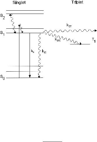
Tissue Optics: Light Scattering Methods and Instruments for Medical Diagnosis |
119 |
Figure 1.47 Jablonski diagram of molecular energy levels and transition rates. Straight lines, radiative transitions; wavy lines, nonradiative transitions.574
tially polarized fluorescence, which is described by the degree of polarization [see Eq. (1.68a)] as
PFL = (IF − IF )/(IF + IF ) |
(1.186) |
||
or by fluorescence anisotropy573 |
|
|
|
r |
IF − IF |
, |
(1.187) |
|
F = IF + 2IF |
|
|
with IF and IF being the fluorescence intensities of light polarized parallel or perpendicular to the exciting electric-field vector, respectively. Usually, PFL and rF depend on the time interval between excitation and fluorescence detection, since during the lifetime of their excited states, many molecules change their orientation by rotation (“rotational diffusion”). From time-resolved measurements of fluorescence anisotropy, a time constant τr of rotational diffusion can be determined that is correlated with the volume VM of the molecule and the viscosity η of its environment according to
τr = |
ηVM |
, |
(1.188) |
kBT |
|||
where kB is the Boltzmann constant and T |
|
is the absolute temperature. Time |
|
constants of rotational diffusion of about 13 ns were correlated with a molecular weight of proteins around 50,000 daltons,573 whereas a time constant around
120 |
Optical Properties of Tissues with Strong (Multiple) Scattering |
300 ps was attributed to an aggregated species of a photosensitizing porphyrin (protoporphyrin) with a 1.6 nm diameter.574
At excitation of biological objects by ultraviolet light (λ ≤ 370 nm), fluorescence of proteins as well as of nucleic acids can be observed. Fluorescence quantum yields of all nucleic acid constituents, however, are around 10−4–10−5, corresponding to lifetimes of the excited states in the picosecond time range. Autofluorescence (AF) of proteins is related to the amino acids tryptophan, tyrosin, and phenylalanine with absorption maxima at 280 nm, 275 nm, and 257 nm, re-
spectively, and emission maxima between 280 nm (phenylalanine) and 350 nm (tryptophan).573–575 The protein spectrum is usually dominated by tryptophan.
Fluorescence from collagen or elastin is excited between 300 and 400 nm and shows broad emission bands between 400 and 600 nm with maxima around 400 nm, 430 nm, and 460 nm. In particular, fluorescence of collagen and elastin
can be used to distinguish various types of tissues, e.g., epithelial and connective
tissue.31,92,98,574–581
The reduced form of coenzyme nicotinamide adenine dinucleotide (NADH) is excited selectively in a wavelength range between 330 and 370 nm. NADH is most concentrated within mitochondria, where it is oxidized within the respiratory chain located within the inner mitochondrial membrane, and its fluorescence is an appropriate parameter for detection of ischemic or neoplastic tissues.574,581 Fluorescence of free and protein-bound NADH has been shown to be sensitive on oxygen concentration. Flavin mononucleotide (FMN) and dinucleotide (FAD) with excitation maxima around 380 nm and 450 nm have also been reported to contribute to intrinsic cellular fluorescence.574
Porphyrin molecules, e.g., protoporphyrin, coproporphyrin, uroporphyrin, or hematoporphyrin, occur within the pathway of biosynthesis of hemoglobin, myoglobin, and cytochromes. Abnormalities in heme synthesis, occurring in the cases of porphyrias and some hemolytic diseases, may enhance the porphyrin level within tissues considerably. Several bacteria, e.g., Propionibacterium acnes, or bacteria within dental plaque (biofilm), such as Porphyromonas gingivalis, Pre-
votella intermedia, and Prevotella nigrescens, accumulate considerable amounts of protoporphyrin.582,583 Therefore, acne or oral and tooth lesion detection based
on measurements of intrinsic fluorescence appears to be a promising method. Recently, a number of theoretical computer modeling and experimental stud-
ies of fluorescence intensity distributions accounting for light scattering effects were performed.584–592 In particular, a diffusion theory model of spatially resolved fluorescence from depth-dependent fluorophore concentration was described in Ref. 585. In Ref. 586, three-dimensional epithelial tissue phantoms suitable for fluorescence spectroscopy, collagen cross-linking studies, and cancer diagnosis were presented. Some principle features of near-infrared fluorescence tomography such as three-dimensional image reconstruction from sparse and noisy data sets587 and localization of fluorescent masses deeply embedded in tissue588 were discussed. A few experimental approaches for recovery of scattering free fluorescence from measured fluorescence589 and validation of Monte Carlo modeling of fluorescence
Tissue Optics: Light Scattering Methods and Instruments for Medical Diagnosis |
121 |
in tissues in the UV-visible spectrum590 were developed. Monte Carlo simulations of some practical cases such as the effect of fiber-optic probe geometry on depthresolved fluorescence measurements from epithelial tissues591 and spatial fluorescence distribution in the skin592 were also performed.
At present, various exogenous fluorescing dyes can be applied for probing of cell anatomy and cell physiology.574,593–597 For instance, subcellular localization
of sulfonated tetraphenyl porphines in colon carcinoma cells was studied by spectrally resolved fluorescence imaging.593
In humans, such dyes as fluorescein and indocyanine green are in use for fluorescence angiography or blood volume determination. Novel fluorescent contrast agents for optical imaging of in vivo tumors based on a receptor-targeted dyepeptide conjugate595 and green fluorescent protein596 platforms were recently described. Fluorescence properties of such dyes as albumin blue 633 and 670 in plasma and whole blood were studied.594 Exogenous specific fluorescence markers for in vivo quantitative three-dimensional localization of tumors were studied in Ref. 597.
Fluorescence spectra often give detailed information on fluorescent molecules, their conformation, binding sites, and interaction within cells and tissues. Fluorescence intensity can be measured either as a function of the emission wavelength or of the excitation wavelength. The fluorescence emission spectrum IF(λ) is specific for any fluorophore and is commonly used in fluorescence diagnostics.
For many biomedical applications, an optical multichannel analyzer (OMA) (a diode array or a CCD camera) as a detector of emission radiation is preferable because spectra can be recorded very rapidly and frequently with sequences in
the millisecond range. Fluorescence spectrometers for in vivo diagnostics are commonly based on fiber-optic systems.133,574–577,591 The excitation light of a lamp or
a laser is guided to the tissue (e.g., some specific organ) via fiber using appropriate optical filters. Fluorescence spectra are usually measured either via the same fiber or via a second fiber or fiber bundle in close proximity to the excitation fiber.
Various comprehensive and powerful fluorescence spectroscopies, such as microspectrofluorimetry, polarization anisotropy, time-resolved with pulse excitation and frequency domain, time-grated, total-internal-reflection fluorescence spec-
troscopy and microscopy, the fluorescence resonant energy transfer method, confocal laser scanning microscopy, and their combinations are available now.573–601
These methods allows one to provide the following:
•3D topography of specimens measured in the reflection mode for morphological studies of biological samples
•High resolution microscopy measured in the transmission mode
•3D fluorescence detection of cellular structures and fluorescence bleaching kinetics
•Time-resolved fluorescence kinetics
•Studies of motions of cellular structures
•Time-grated imaging in order to select specific fluorescent molecules or molecular interactions
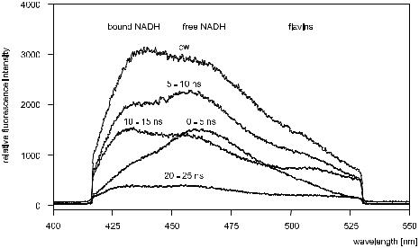
122 |
Optical Properties of Tissues with Strong (Multiple) Scattering |
•Fluorescence lifetime imaging
•Spectrally resolved imaging
The potential of time-gated fluorescence spectroscopy is shown in Fig. 1.48.574,593 Shown fluorescence spectra of Saccharomyces cerevisiae are very
similar to the fluorescence spectra of various cell cultures. An emission maximum at 460–465 nm, corresponding to free NADH, is clearly identified within a time gate of 0–5 ns, whereas emission maxima around 435 nm (bound NADH) and 515 nm (flavins) are resolved at later time gates. In contrast, CW spectra of autofluorescence are broad and exhibit only little substructure.
Figure 1.48 CW and time-gated fluorescence spectra of Saccharomyces cerevisiae after excitation at 365 nm (upper curve) and 355 nm (other curves).593
Using time-resolved fluorescence detection, free and bound NADH could be studied separately; time-gated fluorescence spectroscopy includes studies of the tumor-localizing porphyrins within tissues of strong autofluorescence; and the fluorescence energy transfer method can be used to selectively measure mitochondrial depolarization, which may precede mitochondrial autophagy, apoptosis, and necrotic cell death.574 Analytical models and solutions for time-resolved fluorescence lifetime quantitative spectroscopy and imaging in turbid media and tissue were recently developed.598–601
Principles of optical clinical chemistry based on the measuring of changes of fluorescence intensity, wavelength, polarization anisotropy, and lifetime are described in Ref. 573. Various fluorescence techniques of selective oxygen sensing and blood glucose and blood gases detection are available.573
Tissue Optics: Light Scattering Methods and Instruments for Medical Diagnosis |
123 |
A few examples of fluorescence (autofluorescence) imaging and spectroscopy of normal and pathological tissues such as normal and malignant mucosa in patients with head and neck cancer,602 carotid atherosclerotic plaque,603 cervical precancerous tissue,604 normal and neoplastic human breast tissue,605 and basal cell carcinomas in the skin606 should be mentioned. A real-time calibrated autofluorescence technique for in vivo imaging of neoplastic growths was realized.607 Autofluorescence-based methods and instruments designed for ophthalmic diagnostics are overviewed in Ref. 608.
Currently, reflectance and fluorescence spectroscopies are probably the most developed among the available optical methods for investigating skin in vivo. Reflectance and fluorescence from skin carry information on the structure of epidermis and dermis, on the quantity and density of blood vessels, on the concentration and spatial distribution of chromophores and fluorophores in skin, and on the nature of skin metabolic processes. Typical applications include the in vivo quantitative analysis of skin erythema and pigmentation, determination of cutaneous color vari-
ation, monitoring of dermatological treatment effects, determination of skin photoaging, diagnosis of skin tumors, and study of skin biophysics.57,575,578–580,606
The absorption and scattering properties of the skin affect both the AF and the reflectance spectra. Therefore, the combined use of fluorescence and reflectance may provide additional information for the analysis of skin tissue. The potential advantages and possible uses of the combined use of reflectance and fluorescence spectroscopy of skin for the evaluation of the erythema and pigmentation indices, the determination of the hemoglobin oxygenation and concentration, and the investigation of the efficacy of topical sunscreens are discussed in Ref. 575.
One of the goals of fluorescence spectroscopy is the identification of excitation wavelengths suitable for the differentiation of various pathological conditions. This is closely related to the identification of the chromophores responsible for this differentiation. Most of the biological components, which are either related to the skin tissue structure or are involved in metabolic and functional processes, generate fluorescence emission in the UV-visible spectral region. As a result, different morphofunctional conditions of the skin related to histological, biochemical, and physiochemical alterations can be characterized, in principle, on the basis of
information available in the fluorescence excitation-emission maps (EEMs) (see Fig. 1.49).575,577,579 The fluorescence maximum in the range 320–370 nm with the
peak at 340 nm arises with excitation in the 250–290 nm range (peak at 280 nm). AF in the UVA range is dominated by the fluorescence bands of aromatic amino acids, namely, tyrosine and tryptophan. There is only a slight variation in the UVA fluorescence of the skin between different skin sites. This may be attributed to the absence of AF attenuation by melanin, which is deposited mainly within the epidermis. Tyrosine and tryptophan content in epidermis is more than twice that of the whole skin, and this is why epidermis has a high AF in the UVA range.
Among the endogenous skin fluorophores are also different forms of NAD and keratin located in the epidermis and dermal collagen. The reduced (NADH) and oxidized (NAD+) forms of NAD take part in cellular metabolism, and the intensity of their specific fluorescence (fluorescence maxima near 460 nm and 435 nm,

124 |
Optical Properties of Tissues with Strong (Multiple) Scattering |
Figure 1.49 Excitation-emission maps of the in vivo skin AF emission.579
respectively) is used not only for the differential diagnostics of the metabolism dysfunction, but also in quantitative NADH detection.575
For collagen and elastin, which are located predominantly within the papillary and reticular layers of dermis, both excitation and emission light is attenuated because of absorption by melanin and fluorescence intensity in the 400– 480 nm range is subject to attenuation by other skin chromophores: hemoglobin, porphyrins, carotenoids, etc. Both the total intensity and the spectral features may be affected. The AF spectrum of human skin and the fluorescence spectrum of col-
lagen are essentially identical following optical filtering through the dermal blood plexus.575,580 Figure 1.50 represents the temporal dynamics of the AF skin spec-
tra involved in the process of the UV-erythema formation. The main part of the change observed is a significant decrease of the AF intensity during the erythema formation caused by the optical filtering effect of blood (early stage) and induced melanin (latter stage).
1.7.2 Multiphoton fluorescence
A new direction in laser spectroscopy and imaging of biological objects is associated with multiphoton (twoand three-photon) fluorescence scanning microscopy, which makes it possible to image functional states of an object or, in combination
with autocorrelation analysis of the fluorescence signal, determine the intercellular motility in small volumes.114,122,131,137,609–618 The two-photon technique employs
both ballistic and scattered photons at the wavelength of the second harmonic of incident radiation coming to a wide-aperture photodetector exactly from the focal area of the excitation beam (see Fig. 1.51).609 A unique advantage of two-photon microscopy is the possibility of investigating three-dimensional distributions of
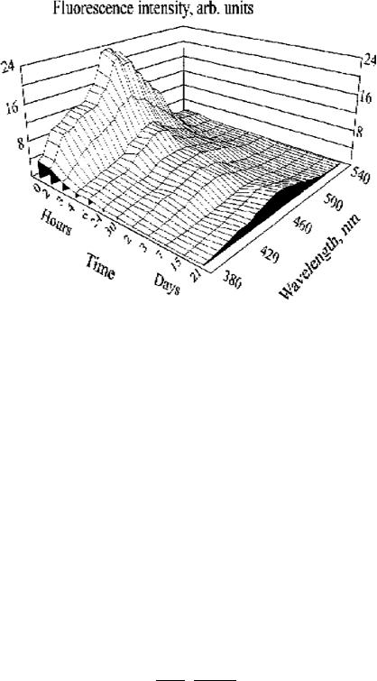
Tissue Optics: Light Scattering Methods and Instruments for Medical Diagnosis |
125 |
Figure 1.50 3D plot of human skin AF after UV irradiation with four minimal erythema doses (MEDs).575,580
chromophores excited with ultraviolet radiation in thick samples. Such an investigation becomes possible because chromophores can be excited (e.g., at the wavelength of 350 nm) with laser radiation whose wavelength falls within the range (700 nm) where a tissue has a high transparency. Such radiation can reach deeply lying layers and produces less damage in tissues. Fluorescent emission in this case lies in the visible range (>400 nm) and comparatively easily emerges from a tissue and reaches a photodetector, which registers only the legitimate signal from the focal volume without any extraneous background.
In a two-photon excitation process, the rate of excitation is proportional to the average squared photon density. This quadratic dependence follows from the requirement that the fluorophore must simultaneously absorb two photons per excitation process. Multiphoton absorption processes are shown in Fig. 1.52. To demonstrate that a multiphoton excitation process has occurred, it is necessary to measure the intensity of fluorescence as a function of the intensity of the excitation light. A two-photon excitation process is characterized by a slope of two on a log-log plot of measured intensities; a three-photon excitation process is characterized by a slope of three.
The rate of two-photon excitation can be described analytically as614
P 2σf π(NA)2 2
n2f ≈ 0 2 , (1.189)
τpfp hcλ
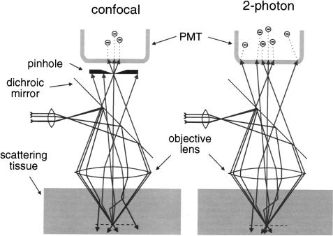
126 |
Optical Properties of Tissues with Strong (Multiple) Scattering |
Figure 1.51 Confocal one-photon excitation imaging compared with two-photon imaging in scattering tissue.609 Because of the longer wavelength, less excitation light is lost to scattering when using two-photon excitation. Ballistic and diffusing fluorescence photons can be used in the two-photon case, but only ballistic photons can be used in the confocal case.
where τp is the pulse duration, fp is the repetition rate, P0 is the average incident power, σf is the photon absorption cross section, h is Planck’s constant, c is the speed of light, NA is the numerical aperture of the focusing lens, and λ is the wavelength. This rate is expressed as the number of photons absorbed per fluorophore per pulse and is a function of the pulse duration, the pulse repetition rate,
the photon absorption cross section, and the numerical aperture of the microscope objective that focuses the light.137,614 The derivation of this equation assumes neg-
ligible saturation of the fluorophore and that the paraxial approximation is valid. The laser light in a two-photon excitation microscope is focused by the micro-
scope objective to a focal volume. Only in this focused volume is there sufficient intensity to generate appreciable excitation. The low photon flux outside the focal volume results in a negligible amount of fluorescence signal. The origin of the optical sectioning capability of a two-photon excitation microscope is due to the nonlinear quadratic dependence of the excitation process and the strong focusing capability of the microscope objective. Most specimens are relatively transparent to near-infrared light. The focusing of the microscope objective results in twophoton excitation of ultraviolet absorbing fluorophores in a small focal volume. It is possible to move the focused volume through the thickness of the sample and
Tissue Optics: Light Scattering Methods and Instruments for Medical Diagnosis |
127 |
Figure 1.52 Multiphoton fluorescence. Diagram showing the absorption and fluorescence processes for a molecule with (a) one-photon absorption, (b) two-photon absorption, and
(c) three-photon absorption. The solid and dashed horizontal lines represent, respectively, real and virtual molecular energy states; the solid vertical arrows, photon absorption pathways; and wavy arrows, fluorescence.
thus achieve optical sectioning in three dimensions. Thus, the optical sectioning in a two-photon excitation microscope occurs during the excitation process.
Investigations of tissues and cells by means of two-photon microscopy are characterized by the following typical parameters of laser systems: the wavelength ranges from 700 to 960 nm, the pulse duration is on the order of 150 fs, the pulse repetition rate is 76–80 MHz, and the mean power is less than 10 mW. Such parameters can be achieved with mode-locked dye lasers pumped by a Nd:YAG laser or with titanium sapphire lasers pumped by an argon laser. Diode-pumped solidstate lasers also hold much promise for the purpose of two-photon microscopy.609 Virtually the same parameters of lasers are required for three-photon fluorescence microscopy of tissue, which possesses the same advantages as two-photon microscopy but ensures a somewhat higher spatial resolution and provides an opportunity to excite chromophores with shorter wavelengths.612
1.7.3 Vibrational and Raman spectroscopies
Middle and far infrared (IR) and Raman spectroscopies use light-excited vibra-
tional energy states in molecules to get information about the molecular composition, molecular structures, and molecular interactions in a sample.30,99,104, 105,115,123,143,619–629 In Fig. 1.53, the IR and Raman processes are depicted in a
molecular energy level diagram. In IR-spectroscopy infrared light from a broadband source [usually in the wavelength range of 2.5–25 μm or in wavenumbers (1/λ) of 4000–400 cm−1] is directly absorbed to excite the molecules to higher vibrational states.624 When the absorbed energy hν matches the energy needed
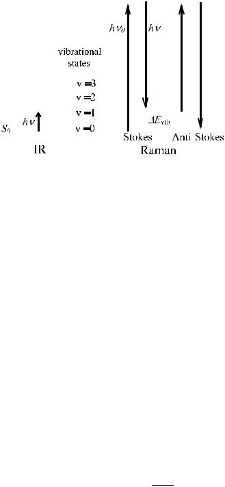
128 |
|
|
|
|
Optical Properties of Tissues with Strong (Multiple) Scattering |
||||||||||||||||
|
|
|
|
|
|
|
|
|
|
|
|
|
|
|
|
|
|
|
|
|
|
|
|
|
|
|
|
|
|
|
|
|
|
|
|
|
|
|
|
|
|
|
|
|
|
|
|
|
|
|
|
|
|
|
|
|
|
|
|
|
|
|
|
|
|
|
|
|
|
|
|
|
|
|
|
|
|
|
|
|
|
|
|
|
|
|
|
|
|
|
|
|
|
|
|
|
|
|
|
|
|
|
|
|
|
|
|
|
|
|
|
|
|
|
|
|
|
|
|
|
|
|
|
|
|
|
|
|
|
|
|
|
|
|
|
|
|
|
|
|
|
|
|
|
|
|
|
|
|
|
|
|
|
|
|
|
|
|
|
|
|
|
|
|
|
|
|
|
|
|
|
|
|
|
|
|
|
|
|
|
|
|
|
|
|
|
|
|
|
|
|
|
|
|
|
|
|
|
|
|
|
|
|
|
|
|
|
|
|
|
|
|
|
|
|
|
|
|
|
|
|
|
|
|
|
|
|
|
|
|
|
|
|
|
|
|
|
|
|
|
|
|
|
|
|
|
|
|
|
|
|
|
|
|
|
|
|
|
|
|
|
|
|
|
|
|
|
|
|
|
|
|
|
|
|
|
|
|
|
|
|
|
|
|
|
Figure 1.53 Illustration of an IR absorption process and a Raman scattering process in a molecular energy level diagram.624
for an allowed infrared excitation of a molecular vibration, an absorption peak is observed in the IR spectrum.
In a Raman scattering event, light is inelastically scattered by a molecule when a small amount of energy is transferred from the photon to the molecule (or from the molecular to the photon). This leads to an excitation of the molecule from usually its lowest vibrational energy level in the electronic ground state S0 to a higher vibrational state of the same electronic state. The Raman spectrum displays the intensity of scattered light as a function of the difference in frequency between the scattered and the incident light. Since each molecular species has its own unique set of molecular vibrations, the Raman spectrum of a particular species consists of a series of peaks or bands of scattered light, each shifted from the incident light frequency by one of the characteristic vibrational frequencies of that molecule. The energy (frequency) difference between incident (hν0) and scattered photon (hν) is expressed as a wave-number shift:624
˜ |
= |
λ0 |
− λ |
|
||
k |
|
1 |
|
1 |
. |
(1.190) |
|
|
|
||||
When the energy of the Raman scattered photons is lower than the energy of the incident photons, the process is called Stokes-Raman scattering. When a photon interacts with a molecule in a higher vibrational level, anti-Stokes Raman scattering can occur, in which the energy of the Raman scattered photons is higher than the energy of the incident photons (see Fig. 1.53). The intensity ratio of the anti-Stokes (IAS) and Stokes (IS) Raman lines for a given vibrational state is given by624
IAS |
|
(ν0 |
+ |
νvib)4 |
hνvib |
, |
|
|
= |
|
|
exp − kB T |
(1.191) |
||
IS |
(ν0 |
− |
νvib)4 |
||||
|
|
|
|
|
|
|
Tissue Optics: Light Scattering Methods and Instruments for Medical Diagnosis |
129 |
where Evib = hνvib is the energy of the molecular vibrational state. It follows that at room temperature the intensity of Stokes-Raman lines in the most informative spectral region (>400 cm−1) is much higher than that of the anti-Stokes-Raman lines. In its turn, the intensity of Stokes-Raman scattered light is very low, typically 10−7 to 10−15 times the intensity of the excitation light. The real-time detection of Raman scattering spectra became practical because of the commercial development of lasers and subsequent advances in detector technology.
Different selection rules apply for excitation of molecular vibrational states
through absorption of an IR photon or through Raman scattering of an incident photon.115,123,621,624 Some vibrations can be excited by both Raman and IR
processes; others can only be excited by either a Raman scattering process or by IR absorption. For symmetric molecules, the selection rules are mutually exclusive for all vibrations. Molecules exhibit IR activity when, during the vibration, a change in the molecular dipole moment occurs. Raman activity occurs when there is a change in polarizability. Therefore, the band intensity in IR and Raman spectra of the same molecular vibrational frequency can be quite different; symmetric vibrational modes are often strong in Raman, whereas antisymmetric vibrational modes are strong in IR. Depending on the polarization state of the incident and observed light, information on the symmetry of the molecules can be obtained.
In most tissues, the fluorescence cross section, when excited by visible or near UV wavelengths (within 300–700 nm), is about six orders of magnitude stronger
than the Stokes Raman cross section; moreover, the fluorescence is a broadband signal within the same spectral range as the Stokes-Raman spectrum.143,624 Fortu-
nately, at different excitation wavelengths, UV, visible, and NIR, Raman scattering produces the same change in vibrational energy, while NIR light has a frequency too low to excite fluorescence and UV-excitated fluorescence has much lower frequency than the Raman scattered light frequency. Hence, the usage of NIR or UV excitation can reduce fluorescence background in the Raman spectrum. Especially for tissue studies, NIR excitation is preferable due to the high penetration depth.
The IR and Raman spectroscopy techniques are successfully applied in various areas of clinical studies such as cancerous tissues examination, the mineralization process of bone and teeth tissue monitoring, glucose sensing in blood, noninvasive diagnosis of skin lesions on benign or malignant cells, and monitoring of treat-
ments and topically applied substances (e.g., drugs, cosmetics, moisturizers, etc.)
in skin.30,99,104,105,143,619,620,622–626
Raman spectroscopy is widely used in biological studies, ranging from stud-
ies of purified biological compounds to investigations at the level of single cells.621,623,625,627,629 At present, combinations of spectroscopic techniques such
as IR and Raman with microscopic imaging techniques are explored to map mole-
cular distributions at specific vibrational frequencies to locally characterize tissues or cells.620,623,624,629 Spectral biochemical imaging will become more and more
important in the clinical diagnosis; in particular, for differentiation of cancerous and noncancerous cells. The measured IR spectra depend on various aspects of sample preparation, i.e., the degree of hydration and homogeneity, and on the phys-

130 |
Optical Properties of Tissues with Strong (Multiple) Scattering |
iological state of cells (exponential phase of growth or plateau); therefore, measurements accounting for named artifacts and cell status should be provided.629 As it was shown recently, the accurate measurement of vibrational spectra of mammalian cells is possible for the homogeneous aqueous cell suspensions; these IR spectra can be closely reproduced with a linear combination of DNA, RNA, phospholipid, glycogen, and protein spectra.629
Because of a penetration depth of middle IR (MIR) light in tissue to only a few micrometers, the attenuated total reflectance Fourier transform infrared spectroscopy (ATR-FTIR) method is suited to study changes of the outermost cell layers of the tissue.624 As an example, sequential hydrated-human-skin stratumcorneum ATR-FTIR spectra measured during occlusion each minute for half an hour are shown in Fig. 1.54. Hydration of the skin is obtained by keeping the forearm pressed against the ATR-FTIR crystal. During occlusion, water in the skin cannot evaporate and accumulates in the skin stratum corneum.
Figure 1.54 Sequential hydrated-human-skin stratum-corneum MIR ATR-FTIR spectra measured during occlusion each minute for half an hour.624 The thick line represents the water spectrum (scaled twice). Spectral changes can be clearly identified: increased contribution of the water-bending mode at 1640 cm−1 and pronounced increase of the OH stretches in the high wave number band around 3300 cm−1. Also, the water combination band around 2125 cm−1 is clearly visible in the hydrated spectra. A Nicolet-800 Fourier Transform spectrometer with a “high-top” model ATR with a ZnSe (n = 2.42) crystal of rectangular shape (10 × 80 mm) with 45-deg entrance and exit facets is used to record spectra. The ATR-FTIR spectrum is obtained by the Fourier transform of 64 and 128 interferograms. The acquisition time for 64 scans at a resolution of 8 cm−1 is about 20 s. Spectra were recorded on the volar part of the forearm by slight pressure on the ZnSe crystal.

Tissue Optics: Light Scattering Methods and Instruments for Medical Diagnosis |
131 |
The Raman technique possesses certain characteristics that make it particularly suitable for studying the skin, both in vitro and in vivo.622,624 In vivo confocal
Raman spectra of the skin show a considerable decrease in the absolute signal intensity if the distance from the laser focus to the skin surface is increased. This is mainly due to diffuse light scattering, which is a much stronger effect in the skin than light absorption. Confocal detection is therefore particularly useful in the study of outer skin layers, i.e., the stratum corneum and the viable epidermis. The in vivo Raman signal of the dermis is strongly reduced due to scattering in the epidermis; therefore, the dermis requires considerably longer signal collection times than for the epidermis. However, since the dermis is much thicker than the epidermis (1–4-mm thick), it can easily be studied using a nonconfocal detection scheme with a detection volume that is large compared to the thickness of the epidermis. In this case, the dermis will be the dominant source of the Raman signal, which is illustrated by Fig. 1.55.624 The figure shows the confocal spectrum measured using a confocal spectrometer and a nonconfocal spectrum measured with a fiber-optic probe. Both spectra were scaled to equal intensity. It is clear that the spectrum obtained with the fiber-optic probe is almost entirely determined by the Raman signal of the dermis. For equal signal collection time, the SNR of the dermis spectrum obtained with the fiber-optic probe is considerably higher than that of the spectrum that was measured confocally.624
Figure 1.55 In vivo Raman spectra of the dermis, as obtained by confocal detection and by nonconfocal detection (fiber-optic probe). Experimental conditions for the confocal spectrum and the nonconfocal spectrum: signal collection time 2 min, laser power 100 mW. The spectra are scaled to equal intensities.624
Near-infrared Raman spectroscopy also has a number of advantages in in vivo detection of cervical tissue pathologies, in particular precancer predictions.30,626
132 |
Optical Properties of Tissues with Strong (Multiple) Scattering |
Surface-enhanced Raman scattering (SERS) is based on a strong increase in Raman signals from molecules if those molecules are attached to submicron metallic
structures. Two effects are believed to contribute to the SERS enhancement mechanisms: electromagnetic effects and chemical effects.620,627 For a smooth metal
surface, there is only a small (on the order of 10 times or less) enhancement of Raman intensity compared with that in the absence of the surface, but for a rough surface due to excitation of electromagnetic resonances by the incident radiation, such enhancement may be of a few orders. These resonances appear due to collective excitation of conduction electrons in the small metallic structures and are also called surface plasmon resonances. Both the excitation and Raman scattered fields contribute to this enhancement; thus, the SERS signal is proportional to the fourth power of the field enhancement factor.620
The surface roughening effect can be achieved by isolated metal particles, by gratings, by assemblies of particles on surfaces, and randomly roughened surfaces. All these structures provide enhancement if the metal involved has narrow plasmon resonances at convenient frequencies for Raman measurements.627 The “chemical mechanisms” include enhancements that arise from interactions between molecule and metal. The most commonly considered interaction that requires overlap between molecular and metal wave numbers occurs when charge transfer between the
surface and molecule leads to the formation of excited states that serve as resonant intermediates in Raman scattering.620,627 Interactions that do not require overlap
between molecular and metal wave numbers arise from electromagnetic coupling between the vibrating molecule and the metal. These interactions can occur either at the vibrational frequency or at optical frequencies. The combined enhancement factors can be as high as 1014, which is enough to observe SERS spectra from single molecules.
1.8 Tissue phantoms
1.8.1 Introduction
Phantoms that model the transport of visible and infrared light in tissue are needed
to evaluate techniques, to calibrate equipment, to optimize procedures, and for
quality assurance.31,46,47,93–95,219,220,233,236,237,263,277,284,467,494,495,511,572,630–646
They have been used in all fields of optical diagnostics, particularly for testing
instruments for timeand frequency-domain transillumination tomography284,639 and spatially resolved reflectance measurements,46,93,637,638 to evaluate the fluorescence spectroscopic technique,632,633,636,641–643 and to test theoretical predictions experimentally.47,94,95,219,220,634,636 Tissue models have been developed for tissue noninvasive glucose monitoring,339–341,535,536,540,541,630,631,635 oxygenation monitoring and oxymetry,516,644 optoacoustics,467,511,516,535,536,540,541 pulsed photothermal measurements,491,495,497 and measuring of polarization degree decay.374,645 Tissuelike phantoms have also been taken up in areas of research
connected with therapeutic implementation of optical radiation, among them being light dosimetry,646 laser ablation,511 and PDT.640,646
Tissue Optics: Light Scattering Methods and Instruments for Medical Diagnosis |
133 |
1.8.2 Concepts of phantom construction
To describe the concepts of constructing phantoms, we will draw upon Refs. 632–
634 and 636. Phantoms consist of a scattering medium, an absorbing medium, a diluent, and in some cases fluorophores.632,633,636 Some common scattering media
are Intralipid, Nutralipid, and Liposyn. These intravenously administered nutrients are fat emulsions that contain soybean oil, egg phospholipids, and glycerol. Other common scatterers are milk or micron-sized latex (polystyrene) spheres. Polystyrene microspheres exhibit low fluorescence, and some of their optical properties can be calculated from Mie theory. Absorbing media include some biological stains such as trypan blue, Evans blue, indocyanine green, methylene blue, and Photofrin II, as well as black India ink. The diluent is usually deionized water, although isotonic phosphate-buffered saline has been used.
An optical phantom is developed by mixing the correct proportions of the scattering and absorbing media in the diluent, so that the resulting suspension has the desired intrinsic optical properties of the simulated tissue. These optical properties include the absorption coefficient μa, the scattering coefficient μs, and the anisotropy factor g. For soft tissues, typical optical properties are μa ≈ 0.5 to 5.0 cm−1, μs ≈ 0.2 to 400 cm−1, and g = 0.9 for visible and NIR wavelengths (see Table 2.1).
A liquid phantom system is very easy to prepare; however, it cannot be used to make samples of realistic complexity. Solid phantom samples have been made using either transparent hosts, such as polymers, silicone, or gelatin; or using inherently light-scattering materials, such as wax. Polymer-based phantoms have been reported to crack if they are too large or to shrink during polymerization, which limits their applicability. Gels contain a solvent that evaporates, changing the dimensions and optical properties of the sample within a short period of time.
Steps toward realistic complex geometries have been the application of
layered samples, inserted inhomogeneities, and phantoms mimicking whole organs.46,47,93–95,233,236,237,277,284,632–636 Some phantom systems have realistic optical properties over a wide wavelength range.47,94,95,236,237 When the task is to
model tissue with complex architecture, or even a whole organ, or to prepare the test object for evaluation of imaging techniques, the “macroscopic” geometry of the natural object should be reproduced in phantom. One of the most commonly en-
countered features is a layered tissue structure. Multilayered phantoms have been developed in the past to mimic, for example, the skin,497 the human head,647,648 and the cervix.641–643
A realistic tissue phantom should satisfy the following requirements:632,633
•It should model the geometry and optical parameters of the physiological structures that are relevant for the transport of light.
•All components must be compatible with each other regarding chemical stability and spectroscopic properties.
•The relevant parameters of radiation transport must be both reproducible and predictable from the sample composition.
134 |
Optical Properties of Tissues with Strong (Multiple) Scattering |
•The physical parameters of the phantom sample should be temporally stable (evaporation, diffusion, aging) and independent of environmental influence.
•The phantom should allow the construction of inhomogeneous samples by stacking phantom slabs or by elaborate molding techniques.
•Sample preparation should be simple, quick, and safe.
The strategy for systematic design of tissue phantom systems showing realistic
optical properties over a broad wavelength range is based on the discrete particle model of tissue.632,633 Light scattering and absorption of particles composing tis-
sue (phantom) are calculated by Mie theory. The relevant parameters are the size (radius a) and shape of the particles; their complex refractive index
n |
(λ |
0 |
) |
= |
n |
(λ |
0 |
) |
+ |
in |
(λ |
0 |
), |
(1.192) |
s |
|
|
s |
|
|
s |
|
|
|
the refractive index of the dielectric host (ground material) n0(λ0), and the relative refractive index of the scatterers and the ground materials, m = ns/n0; λ0 is the wavelength in a vacuum. The imaginary part of the complex refractive index of scatterer material is responsible for light losses due to absorption. Mie theory yields the absorption and scattering efficiencies and the phase function from which the absorption and scattering coefficients, μs = ρσsca and μa = ρσabs, and the scattering anisotropy factor g are calculated; ρ is the scatterers (particles) density. In the framework of Mie theory, the expressions for the scattering and the absorption cross sections can be written in the form148
|
|
|
|
|
|
|
|
|
|
|
|
|
|
λ2 |
∞ |
|
|
|
+ |
|
|
|
| | + | | |
|
|
|
|
|
|
|
|
|
||||||||||||
|
|
|
|
|
|
|
|
|
|
|
|
= 2πn02 |
n 1 |
|
|
|
|
& |
' |
|
|
|
|
|
|
|
|
|||||||||||||||||
|
|
|
|
|
|
|
|
|
|
|
|
|
|
|
0 |
$ |
|
|
|
|
|
|
|
|
|
2 |
|
|
|
|
|
2 |
|
|
|
|
|
|
|
|
||||
|
|
|
|
|
|
|
|
|
σ |
|
|
|
|
|
|
(2n |
|
1) |
|
|
a |
n |
|
|
|
|
|
|
b |
n |
, |
|
|
|
|
|
(1.193) |
|||||||
|
|
|
|
|
|
|
|
|
|
sca |
|
|
|
|
= |
|
|
|
|
|
|
|
|
|
|
|
|
|
|
|
|
|
|
|
|
|
|
|
|
|
|
|||
|
|
|
|
|
|
|
|
|
|
|
|
|
|
|
|
|
|
|
|
|
|
|
|
|
|
|
|
|
|
|
|
|
|
|
|
|
|
|
|
|
|
|
|
|
|
|
|
|
|
= |
|
|
λ2 |
|
∞ |
|
+ |
|
|
|
|
+ |
|
|
|
|
− | |
|
|
| |
|
+ | |
|
| |
|
|
|
|
|
|
|||||||||
|
|
σ |
|
2πn02 |
n 1 |
|
1) Re(a |
|
b ) |
a |
2 |
b |
2 |
|
, |
(1.194) |
||||||||||||||||||||||||||||
|
|
|
|
|
|
0 |
|
(2n |
|
|
|
|
|
& |
|
|
|
|
|
|
|
|||||||||||||||||||||||
|
|
|
|
abs |
|
|
|
|
|
|
|
$ |
|
|
|
( |
|
|
n |
|
|
n |
|
|
|
|
|
|
n |
|
|
|
|
n |
|
|
|
') |
|
|
|
|||
|
|
|
|
|
|
|
|
|
|
|
|
= |
|
|
|
|
|
|
|
|
|
|
|
|
|
|
|
|
|
|
|
|
|
|
|
|
|
|
|
|
|
|
|
|
|
= |
|
|
λ2 |
|
|
|
∞ |
|
|
|
|
|
|
|
|
|
∞ |
|
|
n + 1 |
|
|
|
|
|
|
|
+ + |
+ |
|
|
||||||||||||
g |
πn02σsca n 1 n(n + 1) |
|
|
|
+ n 1 |
|
|
|
|
|
|
|
|
|
||||||||||||||||||||||||||||||
|
|
|
|
0 |
|
|
$ |
2n + 1 |
Re(anb ) |
|
$ |
n(n + |
|
2) Re ana |
|
|
|
bnb |
|
, |
||||||||||||||||||||||||
|
|
|
|
|
|
|
|
|
|
|
|
|
n |
|
|
|
|
|
|
|
|
|
|
|
|
|
|
& |
n |
|
|
1 |
|
n |
1 |
' |
||||||||
|
|
|
|
|
|
|
|
= |
|
|
|
|
|
|
|
|
|
|
= |
|
|
|
|
|
|
|
|
|
|
|
|
|
|
|
|
|
|
|
|
|
|
|
|
|
(1.195) where an asterisk indicates the complex conjugate; and an and bn are Mie coefficients, which are functions of the relative complex refractive index of particles (m) and parameter 2πan0/λ0 to be taken as
|
ψn(α)ψ |
(mα) |
− |
mψn(mα)ψ |
(α) |
|
|||
a |
n |
|
|
n |
|
, |
(1.196) |
||
ξ(α)ψn(mα) |
|
|
|
|
|||||
n = |
− |
mψn(mα)ξn(α) |
|
||||||
|
|
|
|
|
|
|
|
||

Tissue Optics: Light Scattering Methods and Instruments for Medical Diagnosis |
135 |
|
|
mψ (mα)ψn(α) |
− |
ψn(mα)ψ |
(α) |
|
||||
b |
|
|
|
|
|
n |
|
, |
(1.197) |
|
n = mψn(mα)ξn(α) |
− |
|
|
|
||||||
|
ψn(mα)ξn(α) |
|
||||||||
|
|
|
|
|
|
|
|
|
||
|
|
m = |
np |
; α |
= |
2πan0 |
, |
|
|
(1.198) |
|
|
n0 |
λ0 |
|
|
|||||
where a is the radius of spherical scattering particles, λ0 is the light wavelength in vacuum, ψn, ξn, ψn, ξn are the Riccati-Bessel functions of the first or second kind, n0 is the refractive index of the ground (host) material, and np is the refractive index of scattering particle material.
The introduction of the specific scattering and absorption coefficients extrap-
olated to a volume fraction of 100% is useful for describing scattering and absorption properties of the medium under construction.632,633 In that case and when
the particles are sufficiently diluted to prevent dependent scattering, the scattering, transport scattering, and absorption coefficients are proportional to the dimensionless volume fraction of scatterers cs,
μs = cs |
|
sca, μs = cs |
|
sca[1 − g(λ0, a)], μa = cs |
|
abs, |
(1.199) |
σ |
σ |
σ |
where the specific scattering and absorption coefficients σsca and σabs are expressed in cm−1. The optical parameters of broadband particle size distributions are values averaged over the distribution weighted by the volume fractions of particles with different diameters. The relative frequencies of the corresponding particle size are determined from images made with an electron microscope. The resulting specific optical coefficients are the averaged values and can be defined analogously to Eqs. (1.173)–(1.176). The mean distance ds between the centers of gravity of the particles is determined by their radius a and volume fraction cs as
|
|
2a |
|
||
|
= √cs |
(1.200) |
|||
ds |
|
|
|
. |
|
|
3 |
|
|
|
|
Mie theory predicts that scattering introduced by spherical micrometer-sized particles is strongest if the particle radius and wavelength are of the same order of magnitude. Mie theory is strictly only applicable to particles of particular regular shapes, but results are still useful if the shape is irregular. The oscillatory structure of the scattering coefficient and anisotropy factor as a function of particle size, which is observed with spherical particles (Fig. 1.56), is averaged out.148 The transport scattering coefficient increases strongly with the ratio ns/n0. In turn, the scattering anisotropy factor is maximal when this ratio approaches 1 (Fig. 1.56). A trade-off has to be made between maximizing scattering (to prevent dependent scattering) and optimizing the scattering anisotropy factor when constructing certain phantoms.
For the matched refractive indices of scatterers and background material, the scattering coefficient goes to zero, which means that only absorption is responsible
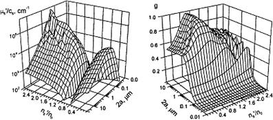
136 |
Optical Properties of Tissues with Strong (Multiple) Scattering |
now for the light beam extinction [see Eq. (1.1)]. However, as it follows from Mie theory, absorbing particles suspended in an index-matched medium cause strongly
forward-directed resonance scattering. Light absorption by such particles is smaller than expected from their bulk absorption coefficient.632,633 For 1-μm diameter par-
ticles with ns = 1.6 and a bulk absorption coefficient of their material equal to
in an index-matched medium, the particle system absorption coefficient μa = cs × 4120 cm−1.
(a) |
(b) |
Figure 1.56 Designing of a tissue phantom. The scattering properties of nonabsorbing particles at a wavelength of 633 nm are calculated by Mie theory.632,633 The transport scattering coefficient (a) strongly depends on both the particle size and relative refractive index. This graph is approximately symmetric. The axis of symmetry is at ns/n0 = 1. While the transparent scattering coefficient equals zero there, in (b) the scattering anisotropy factor is maximal. In some parts of the range shown, the functions are not monotonous, but rapidly oscillating.
The wavelength dependencies of scattering parameters are shown in Fig. 1.57. The spectral variation of the relative index has been neglected in calculations, but may be relevant in practice. If particle size and ratio of refractive indices are fixed, the wavelength dependencies are caused by the spectral variation of the ratio of particle size and wavelength. For particles with a refractive index close to that of the host (see Fig. 1.57), the scattering coefficient of the particle system with a diameter of particles smaller than the wavelength decreases with wavelength, while that of the system with a diameter of particles larger than the wavelength is almost constant. The scattering anisotropy factor depends less on the wavelength. There are plateaus if the particles are much smaller (isotropic scattering) or larger (highly anisotropic scattering) than the wavelength, with a steep increase between.
Biological tissue shows increasing scattering toward shorter wavelengths and high scattering anisotropy. These cannot be realized using monodisperse particles. Therefore, a mixture of large particles contributing high scattering anisotropy and
small particles with increasing scattering toward shorter wavelengths should be a good approximation for the elaborating of a tissuelike phantom.179,632,633
Tissue Optics: Light Scattering Methods and Instruments for Medical Diagnosis |
137 |
(a) |
(b) |
Figure 1.57 Designing of a tissue phantom. The wavelength dependencies of scattering by nonabsorbing particles at ns/n0 = 1.07 are calculated by Mie theory.632,633 The specific transport scattering coefficient (a) of particles smaller than the wavelength increases strongly toward shorter wavelengths. Particles with a diameter larger than the wavelength have an almost constant specific transport scattering coefficient over the whole visible spectral range. The scattering anisotropy factor (b) scarcely depends on the wavelength, but very much on the particle size.
1.8.3 Examples of designed tissue phantoms
Optical phantoms at 1064 nm on the basis of Intralipid and India ink mixtures have been developed using the preliminary experimentally determined absorption coefficient, scattering coefficient, and anisotropy factor of the components.634 For evaluation of the optical parameters of phantom components and phantoms themselves, the integrating sphere technique together with the collimated light transmission measurements and the inverse adding-doubling (IAD) algorithm were used. The average optical properties from all the data for the phantom components are shown in Table 1.6. A comparison of the predicted, measured, and calculated optical properties of the two phantoms are shown in Table 1.7. In Table 1.8, the predicted (Mie theory) and measured (IAD algorithm) data for two phantoms (804-nm diameter polystyrene sphere and water suspensions) are presented.
Table 1.6 Average optical properties in dependence on concentration of India ink, 10% Intralipid, and water at 1064 nm.634
Scattering media |
μs/%, cm−1/% |
μa/%, cm−1/% |
g |
|
India ink |
4.64 |
± 2.07 |
35.99 ± 4.28 |
0.30 ± 0.18 |
Intralipid |
1.30 |
± 0.047 |
0.054 ± 0.02 |
0.50 ± 0.02 |
Water |
– |
|
0.0018 |
– |
Note: The absorption results of Intralipid are corrected for water absorption.

138 |
Optical Properties of Tissues with Strong (Multiple) Scattering |
||
Table 1.7 Predicted and measured optical properties of phantoms.634 |
|||
|
|
|
|
Phantoms |
μs, cm−1 |
μa, cm−1 |
g |
Phantom 1 (Intralipid and India ink) |
|
|
|
Predicted |
8.82 |
0.32 |
0.48 |
Measured |
9.69 ± 0.22 |
0.76 ± 0.01 |
0.56 ± 0.00 |
Calculated |
8.75 |
0.89 |
0.50 |
Phantom 2 (Intralipid only) |
|
|
|
Predicted |
8.82 |
0.00 |
0.48 |
Measured |
8.84 ± 0.03 |
0.33 ± 0.01 |
0.51 ± 0.00 |
Calculated |
8.70 |
0.53 |
0.50 |
|
|
|
|
Note: The predicted values for phantoms 1 and 2 assume that Intralipid and water do not absorb and that ink does not scatter 1064-nm light. The calculated values were determined from the concentration values found in Table 1.6.
Table 1.8 Predicted and measured optical properties of phantoms (804-nm diameter polystyrene sphere and water suspensions) at 1064 nm.634
Phantoms |
μs, cm−1 |
μa, cm−1 |
g |
Phantom 1 |
|
|
|
Predicted |
2.23 |
– |
0.807 |
Measured |
1.99 ± 0.12 |
0.28 ± 0.02 |
0.775 ± 0.04 |
Phantom 2 |
|
|
|
Predicted |
2.96 |
– |
0.807 |
Measured |
3.15 ± 0.01 |
0.25 ± 0.01 |
0.811 ± 0.004 |
Note: The predicted values for phantoms 1 and 2 were calculated using the Mie theory. The absorption coefficients were not corrected for water absorption.
All these data clearly show that liquid phantom systems allow the design of controlled tissuelike phantoms and their optical properties on at least one wavelength are well predicted theoretically. In particular, by knowing the dependence of scattering and absorption of the India ink and Intralipid, a phantom with predicted optical properties can be constructed. However, the constructed phantom’s final optical properties should be measured for an accurate determination of phantom optical parameters. Unfortunately, the scattering properties of diluted Intralipid correspond to those of tissues that have a relatively low scattering anisotropy factor of about g = 0.56. A more realistic value of an anisotropy factor can be obtained by water suspensions of polystyrene spheres with a diameter close to the wavelength. A comparison of the constructed phantom’s optical properties at 1064 nm with the corresponding optical parameters of human tissues, presented in Table 2.1, shows that the absorption properties of these phantoms are well matched to many tissues, but the scattering properties are much lower than for tissues.
Tissue Optics: Light Scattering Methods and Instruments for Medical Diagnosis |
139 |
To check the validity of analyzing the optical properties of human skin by using in vivo reflectance measurements, liquid phantoms consisting of Intralipid-10% as a scatterer and Evans blue as an absorber in phosphate-buffered saline were applied.572 Concentrations of Intralipid-10% in the range 10–50% and Evans blue up to 0.01 g/l were used. In an ex vivo study of human skin in the NIR range, phan-
toms composed of aqueous solutions of 1.27-μm polystyrene microspheres and infrared dye (S109564 Zeneca) were used.236,237 The accuracy and the limitations
of the experimental system for spatially resolved absolute diffuse reflectance mea-
surements were tested using tissue-simulating phantoms that consisted of Liposyn20% stock solution and trypan blue dye as the absorber.46,93 For a 1% volume
concentration of Liposyn (without trypan blue) at 633 nm, μs = 14.0 ± 0.5 cm−1, g = 0.8, and μa = 0.005 cm−1 were found.
Comparing the experimental results for absorption length, transport length, and anisotropy factor against wavelength obtained for a 2% Intralipid-10% stock solution with Mie theory, it was found that one can use the following approximations:31,92
μ |
(λ) |
≈ |
1.6 |
× |
103 |
λ−1 |
(cm−1) and g(λ) |
≈ |
1.1 |
− |
0.58 |
× |
10−3 |
λ, |
(1.201) |
s |
|
|
|
|
|
|
|
|
|
|
for wavelengths from 400 to 1100 nm. To obtain a solution with μs = 76.9 cm−1
and μs = 10 cm−1 at 550 nm, the stock solution of Intralipid-10% was diluted as 1:2 and 1:15, respectively.31,92
Sometimes, in the constructing of phantoms with precise optical properties in a wide range of wavelengths, the dependencies of refractive indices of phantoms’ components should be included. For example, for water-polystyrene suspension phantoms, to include the wavelength dependence of the refractive indices of water
and polystyrene particles, the dispersion functions for water (w) and polystyrene
(p) valid in the visible and NIR should be used as630
nw(λ) = |
1.31848 + |
|
|
|
|
6.662 |
|
|
|
|
|
|
|
|
|
|
|
|||||||||||
λ |
|
nm |
] − |
129.2 |
|
|
|
|
|
|
|
|
|
|
||||||||||||||
|
|
|
|
|
|
|
|
[ |
|
|
|
|
|
|
|
|
|
|
|
|
|
|
|
|||||
|
= |
1.3199 |
+ |
6878 |
− |
|
1.132 × 10⁹ |
|
|
|
1.11 × 10¹⁴ |
. |
(1.202) |
|||||||||||||||
|
|
λ |
|
|
|
|
|
|
|
|||||||||||||||||||
|
|
|
|
2 |
|
|
|
λ |
4 |
|
+ |
λ |
6 |
|
|
|
||||||||||||
|
|
|
|
|
|
|
|
|
|
|
|
|
|
|
|
|
|
|
|
|
|
|
|
|||||
n |
p = |
1.5626 |
+ |
11690 |
|
− |
1.25 × 10⁹ |
+ |
|
1.72 × 10¹⁴ |
, |
|
(1.203) |
|||||||||||||||
|
|
λ2 |
|
|
|
|
|
|
||||||||||||||||||||
|
|
|
|
|
|
|
|
|
|
λ4 |
|
|
|
|
λ6 |
|
|
|
|
|||||||||
where λ is in nanometers.
To study laser-induced stress transients in a nonscattering homogeneously absorbing liquid where a theoretical description of optoacoustic phenomena
is straightforward, an aqueous solution of potassium chromate (K2CrO4) was used.467,511 This solution does not fluoresce, and the total absorbed laser energy is
therefore converted into heat; it is photochemicaly stable, and its optical properties
140 |
Optical Properties of Tissues with Strong (Multiple) Scattering |
are not altered, even at high laser fluences. A solution of 35 mg of K2CrO4 per cubic centimeter yields an absorption coefficient of 1000 cm−1 at 355 nm. Dilution of the initial solution allows one to control the light penetration depth and, therefore, the acoustic frequency of laser-induced stress waves.467
Laser-induced stress generation, propagation, and detection in tissues can be well modeled with the help of turbid absorbing gels.467 A warm water solution (90 cm3) was mixed with 10 g of gelatin powder to prepare gel phantoms. These gels were colored with potassium chromate and made turbid with polystyrene microspheres (0.9 μm in diameter). A 10% polystyrene sphere solution has a scattering coefficient of μs = 6090 cm−1 and an anisotropy factor g = 0.918 at 355 nm, yielding a reduced scattering coefficient of μs = 499 cm−1; the absorption coefficient at 355 nm is defined by the concentration of K2CrO4 and can be very high, up to 1000 cm−1. However, the spectral range of importance for biomedical optics is from visible to NIR, in which diagnostics, imaging, and photodynamic therapy treatments are performed. Therefore, the polystyrene sphere concentration can be chosen to be approximately 2% in the experimental gels, which yields μs = 99 cm−1. A typical μs/μa ratio for biological tissues at 600–1000-nm wavelength is from 70 to 100, which can be easily realized for such phantoms. Soft elastic collagen gel phantoms can be prepared using milk as a scatterer and can be colored with hemoglobin or even whole blood. They allow for easy embedding of inclusions modeling various pathology states (for instance, an absorbing sphere simulating tumor) or modeling the specificity of tissue structure (for instance, a vessel network).
Adding a small percentage of agarose to solidify the well-characterized and easily available water solutions of Intralipid and ink is a good alternative for more complicated solid phantoms.284 Solutions of such phantom consist of 1% agarose in distilled water, with Intralipid and black ink added. The agarose produces a gelatin that can be easily manufactured in order to create and embed an inclusion.
In addition, gelatin (collagen) gel phantoms with different optical properties can be stacked on top of each other to yield a layered-tissue structure model.277,641–643
TiO2 particles can be used as scatterers and India ink can be used as an absorber in the constructing of gelatin (collagen) gel phantoms.
TiO2 particles 0.3 μm in diameter and Projet 900NP dye (Zeneca) were used as
scatterers and absorber in solid phantoms composed of Araldite epoxy resin (Ciba Polymers).236,237 These phantoms also allow one to combine optical properties by
stacking slabs with different optical parameters. As a homogeneous solid scattering phantom for calibration of a microspectrophotometric optical system, a composite consisting of highly dispersed SiO2 particles (diameter < 10 μm, volume-filling fraction, 43%) in an organic methacrylate matrix was used.263
Temporally stable samples were made from a phantom system based on poly-
organosiloxane (POS, silicone) as a host, which has been described in detail elsewhere.632,633 Highly hydrophobic POS is supplied in monomeric form as a
two-component system. It is especially suited to the modeling of fine structures. When a cross-linking component is added, POS starts to polymerize in an additional reaction; it takes typically less than 30 min at 80◦C in a drying oven. There

Tissue Optics: Light Scattering Methods and Instruments for Medical Diagnosis |
141 |
is no shrinking or cracking. Particles as small as 40 nm in diameter are immobilized in the rubber meshwork. The resulting rubber is mechanically stable and transparent in the visible range. Its refractive index equals 1.40 at 589 nm. This method of phantom preparation allows one to construct multilayer phantoms with stepwise varying optical properties without any gap between homogeneous layers, and to include fine tissue details such as structured surfaces and tiny holes, modeling tissue surface and blood vessels, respectively. Various types of particles can be used to induce scattering. Some of them with negligible absorption in the visible spectral region are presented in Table 1.9. This table illustrates the range of values for the relative refractive indices that can be provided in two phantom systems considered.
To achieve homogeneous dispersion, particles should be dispersed in a host media by an ultracentrifuge. The authors of Refs. 632 and 633 used spherical porous
Table 1.9 Relative refractive indices of substances with negligible absorption in the visible spectral range.632,633
Substance |
In aqueous gel |
In POS |
|
|
|
SiO2 |
1.10 |
1.04 |
γ-Al2O3 |
1.20 |
1.14 |
BaSO4 |
1.23 |
1.17 |
MgO |
1.31 |
1.24 |
α-Al2O3 |
1.33 |
1.26 |
TiO2 |
1.95 |
1.86 |
Note: The relative refractive index is given for an aqueous gel (n0 = 1.33) and POS (n0 = 1.40 at 589 nm) for a host. The particles are assumed to be massive.
Table 1.10 Comparison of the results of integrating sphere measurements and Mie calculation based on isolated characterization.632,633
Wavelength, |
Method |
Porous aluminium oxide |
Iron particles |
|
|
|||||
nm |
|
particles |
|
|
|
|
|
|
|
|
|
|
|
|
|
|
|
|
|
|
|
|
|
|
sca, cm−1 |
|
abs, cm−1 |
|
|
sca, cm−1 |
|
abs, cm−1 |
|
|
σ |
σ |
σ |
σ |
|||||
546 |
Mie theory |
210(50)a |
– |
3000(600)c |
4500(900)c |
|||||
546 |
Measured |
200(10)b |
<0.7 |
|
3500(900)a |
3800(200)a |
||||
633 |
Mie theory |
210(50)a |
– |
3000(600)c |
4500(900)c |
|||||
633 |
Measured |
190(10)b |
<0.7 |
|
2800(800)a |
3900(200)a |
||||
Note: The assumption was that the pores of the particles are completely filled with POS and the average refractive index of particles was estimated. Spherical porous aluminium oxide particles have a symmetrical size distribution, with the mean value 5.3 ± 1.0 μm, and spherical iron particles have an asymmetrical size distribution: 16% of the volume fraction is contributed by particles of diameter up to 2.0 μm, 50% by particles up to 3.0 μm, and 84% by particles up to 3.6 μm.
Errors are given in parentheses in units of the last digit(s) and are: a the upper limit error caused by uncertain refractive index (particle composition); b sum of error of measurement, limited reproducibility of sample production, error of sample thickness, and systematic error of diffusion theory; c variations of reported values.
142 |
Optical Properties of Tissues with Strong (Multiple) Scattering |
aluminium oxide, iron, and modified amino resin (MAR) particles to obtain an appropriate scattering. Some data that allow one to compare the optical properties predicted by Mie theory, taking into account the optical properties of isolated particles and their size distributions, and the optical properties of POS phantoms measured using the integrating sphere technique are presented in Table 1.10. These phantoms were designed for modeling the fluorescence of tissue components, in particular, protoporphyrin IX fluorescence.
Various phantoms have been designed to determine the accuracy of in vivo optical monitoring of glucose concentration in blood and tissues.339–341,535,536,540,
541,630,631,635
1.8.4 Examples of whole organ models
Models of whole organs are described in the literature.636,647,648 For example, human skin was modeled by a film (50 to 150 μm) of hydrated Type I collagen.494,495
This film contained variable amounts of subsurface absorbers positioned at a given depth and simulated discrete chromophores buried in multilayered composite human skin. The chromophores were constructed by staining a film with triphenylmethane dye, which absorbs optimally at 585 nm. Discrete chromophores were prepared by cutting a stained collagen film (125-μm thick) with known optical absorption (μa = 400 cm−1) into a number of thin strips (100to 300-μm width). A model skin phantom was constructed by positioning variably spaced (50 to 700 μm) absorbing thin strips underneath a known thickness (110 μm) of a nonabsorbing collagen film. The absorbing thin strips and nonabsorbing films were positioned on a 10-mm thick collagen sponge to simulate an infinite half-space as in living skin.
Another example of whole organ modeling consists of models of the adult head.233,647,648 The models233 consist of threeor four-layered slabs, the latter in-
corporating a clear cerebrospinal fluid (CSF) layer. The most sophisticated model also incorporates slots that imitate sulci on the brain surface. Using these models, it was shown that light propagation in the adult head is highly affected by the presence of the clear CSF layer, and both the optical path length and the spatial sensitivity profile of the models with a CSF layer are quite different from those without the CSF layer. However, the geometry of the sulci and the boundary between the gray and the white matter have little effect on the light distribution detected.