


4
Coherent Effects in the Interaction of Laser Radiation with Tissues and Cell Flows
In this chapter, coherent effects that accompany the propagation of laser radiation in tissues and the interaction of laser radiation with cell flows are considered. These effects include diffraction, formation of speckle structures, interference of speckle fields, scattering from moving particles, etc. Principles of quasi-elastic light scattering (QELS) spectroscopy, diffusion wave spectroscopy (DWS), full-field speckle imaging (LASCA), confocal microscopy, optical coherence tomography (OCT), and second-harmonic generation (SHG) imaging are discussed.
4.1 Formation of speckle structures
Speckle structures are produced as a result of interference of a large number of elementary waves with random phases that arise when coherent light is re-
flected from a rough surface or when coherent light passes through a scat-
tering medium.45,76,77,82,83,112,113,129,136,139,155,157,343,396,821–837 The speckle phe-
nomenon is a three-dimensional interference effect that exists in all points of space where the reflected or transmitted waves from an optically rough surface or volume intersect. Generally, there are two types of speckles: subjective speckles, which are produced in the image space of an optical system (including an eye), and objective speckles, which are formed in a free space and are usually observed on a screen placed at a certain distance from an object. Since the majority of bioobjects are optically nonuniform, irradiation of such objects with coherent light always gives rise to speckle structures that either distort the results of measurements and, consequently, should be eliminated in some way, or provide new information concerning the structure and the motion of a bioobject and its components. In this tutorial, we will mainly discuss the information aspects of speckle fields.
Figure 4.1 schematically illustrates the principles of the formation and propagation of speckles produced in the regime of transmission and reflection of coherent light in an optically nonuniform media; Fig. 4.2 shows a real speckle pattern formed at He:Ne laser beam transmission through a thin layer of a human epidermal sample. The average size of a speckle in the far-field zone is estimated as
dav λ/ϕ, |
(4.1) |
where λ is the wavelength and ϕ is the angle of observation.
289

290 |
Coherent Effects in the Interaction of Laser Radiation with Tissues and Cell Flows |
(a)
(b)
(c)
Figure 4.1 (a) Formation and propagation of speckles, (b) observation of speckles, and
(c) intensity modulation; W is the scattered wave.821
Displacement x of the observation point over a screen or the scanning of a laser beam over an object with a certain velocity v (or an equivalent motion of the object itself with respect to the laser beam) when the observation point remains stationary gives rise to spatial or temporal fluctuations of the intensity of the scattered field. These fluctuations are characterized by the mean value of the intensity I and the standard deviation σI [see Fig. 4.1(b)]. The object itself is characterized by the standard deviation σh of the altitudes (depths) of inhomogeneities and the
correlation length Lc of these inhomogeneities (random relief).
Since many tissues and cells are phase objects,77,343 the propagation of coherent beams in bioobjects can be described within the framework of the model of a random phase screen (RPS).75 The amplitude transmission coefficient of an RPS is given by
Tissue Optics: Light Scattering Methods and Instruments for Medical Diagnosis |
291 |
Figure 4.2 Speckle pattern produced at He:Ne laser beam transmission through a thin human skin epidermal sample (skin epidermal strip).
ts (x, y) = t0 exp{−i (x, y)}, |
(4.2) |
where t0 is the spatially independent amplitude transmission and (x, y) is the random phase shift introduced by the RPS at the (x, y) point. Such spatial phase may be due to variations in the refractive index n(x, y) or the RPS thickness h(x, y) from point to point. For thin transmitting and reflecting RPSs, we have
|
π |
|
|
|
|
(x, y) = |
2 |
{n(x, y) − 1}h(x, y), |
|
||
λ |
|
||||
|
|
|
π |
|
|
(x, y) = |
4 |
h(x, y), |
(4.3) |
||
λ |
|||||
respectively. Phase fluctuations of the scattered field are characterized by the standard deviation σφ and the correlation length Lφ. Generally, there are two types of RPSs: weakly scattering RPSs (σ2φ 1) and deep RPSs (σ2φ 1).
The ideal conditions for the formation of speckles, when completely developed speckles arise, can be formulated in the following manner:
1.Coherent light irradiates a diffusive surface (or a transparency) characterized by Gaussian variations of optical length L = (nh) with the probability density distribution
= , |
|
- |
|
|
− |
2σL2 |
|
|
p( L) 2πσ |
2 |
|
1/2 |
exp |
|
( L)2 |
. |
(4.4) |
|
L |
|
|
|
|
|
|
|

292Coherent Effects in the Interaction of Laser Radiation with Tissues and Cell Flows
2.The standard deviation of relief variations is such that σL λ; both the coherence length of light and sizes of the scattering area considerably exceed the differences in optical paths caused by the surface relief, and many scattering centers contribute to the resulting speckle pattern.
Statistical properties of speckles can be divided into statistics of the first and second orders. Statistics of the first order describe the properties of speckle fields at each point. Such a description usually employs the intensity probability density
distribution function p(I ) and the contrast |
|
|
|||
VI = |
σI |
, |
σI2 = I |
2 − I 2, |
(4.5) |
I |
|||||
where I and σ2I are the mean intensity and the variance of the intensity fluctuations, respectively. In certain cases, statistical moments of higher orders are employed. For example, in addition to contrast, generally defined as
VI = μ1 |
|
1/2 |
(4.6) |
|||
|
, |
|||||
|
μ2 |
|
|
|
|
|
we can introduce the asymmetry parameter |
|
|
|
|
||
Qa = |
μ3 |
|
, |
(4.7) |
||
μ1.5 |
||||||
|
|
|
2 |
|
|
|
which provides additional information concerning the scattering object. Here, the statistical moments are defined as
N |
|
$ |
|
μn = (N − 1)−1 (Ij − μ1)n. |
(4.8) |
j =1
For ideal conditions, when the complex amplitude of scattered light has Gaussian statistics, the contrast is VI = 1 (developed speckles), and the intensity
probability distribution function (PDF) is represented by a negative exponential function as157
p(I ) = |
I |
exp − I . |
(4.9) |
|
|
1 |
|
I |
|
Thus, the most probable intensity value in the corresponding speckle pattern is equal to zero; i.e., destructive interference occurs with the highest probability.
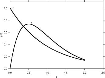
Equation (4.9) is plotted as curve 1 in Fig. 4.3, and it can be seen that the most probable speckle is dark. The intensity PDF described by this equation can be produced only by the interference of light that is polarized all in the same manner,
Tissue Optics: Light Scattering Methods and Instruments for Medical Diagnosis |
293 |
resulting in a similarly polarized speckle pattern.828 Thus, the scattering surface can not depolarize the scattered light. Materials into which the light does not penetrate and is scattered only a single time generally produce speckle patterns that have an intensity distribution in accordance with Eq. (4.9). On the other hand, materials into which the light penetrates and is subject to multiple scattering, such as most biological tissues, tend to depolarize the interfering light.
Figure 4.3 Theoretical intensity probability distribution functions p(I ) of a fully developed speckle pattern [curve 1, Eq. (4.9)] and the incoherent combination of two speckle fields [curve 2, Eq. (4.10)].828
Laser speckle patterns originating from most biological tissues are not “fully developed” in the sense that their intensity distribution does not follow a negative exponential relationship [Eq. (4.9)]. Such speckle patterns may have a distinctly different intensity PDF, one that is best thought of in terms of an incoherent com-
bination of two speckle fields. Many speckle interferometers function by allowing two independent speckle patterns to interfere.157,822–835 The speckle patterns can
interfere either coherently or incoherently. In the case of a coherent combination, the statistical properties of the resulting third speckle pattern remain fundamentally the same as the two original patterns, typically following Eq. (4.9). However, in the case of an incoherent combination of two speckle fields, the final intensity PDF does not obey negative exponential statistics, but instead follows the equation828
p(I ) = 4 II |
2 |
exp − |
I |
. |
(4.10) |
||
|
|
|
|
2I |
|
||
|
|
|
|
|
|
||
The shape of this relationship is shown as curve 2 in Fig. 4.3. The intensity PDF of individual speckle patterns arising from most biological tissues obeys this equation. The reason is as follows: coherent light scattered from most biological tissues
294 |
Coherent Effects in the Interaction of Laser Radiation with Tissues and Cell Flows |
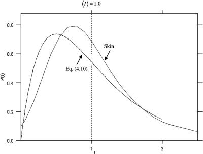
produces randomly polarized speckle patterns, and any two orthogonally polarized components of scattered light are incoherent with one another. Thus, single speckle patterns arising from biological tissues that randomly polarize the speckle pattern can be considered to be the incoherent combination of two or more speckle patterns. Figure 4.4 shows the measured intensity PDF of a backscattered speckle pattern arising from illuminating a sample of porcine skin with an expanded He:Ne laser (633 nm). It is clearly seen that the intensity PDF of the scattered light from the skin more or less follows that predicted by Eq. (4.10).
Figure 4.4 Measured intensity probability distribution function p(I ) of the speckle field generated by illuminating a sample of porcine skin with a He:Ne laser (633 nm) compared to that predicted by an incoherent combination of two fields [Eq. (4.10)].828
Partially developed speckle fields are characterized by a contrast VI < 1. The contrast may be lower for the following reasons:
(1)If a uniform coherent background with intensity Ib is added to the speckle field, then we have
2 |
' |
1/2 |
|
(4.11) |
VI = &1 − ρb |
|
, |
where ρb = Ib /( Ib + I ). For example, with a decrease in the roughness of a surface (or the nonuniformity degree of a solid scatterer), we have σ2φ → 0. Under these conditions, the strong specular (nonscattered) component of the coherent beam interferes with the speckle field. In the limiting
Tissue Optics: Light Scattering Methods and Instruments for Medical Diagnosis |
295 |
case of an ideally plane surface (a uniform medium), speckles vanish and VI = 0.
(2)If a uniform incoherent background (e.g., due to lowering of the coherence of the light source or multiple scattering in the medium) arises, then we have
VI = 1 − ρb. |
(4.12) |
For Gaussian statistics and a Gaussian correlation function of phase fluctuations, the propagation of intensity of the speckle field in a free space along the z-axis behind the RPS is described by the expression75
σI2(z) = |
σφ2 |
|
1 + |
1 + D2 |
' |
− |
1 |
, |
(4.13) |
2 |
|
||||||||
|
|
|
, |
& |
|
|
- |
|
where D = zλ/πL2φ is the wave parameter. For a weakly scattering RPS (σ2φ 1),
the contrast of the speckle field is always less than unity. For a deep RPS (σφ2 1), |
|||||
2 |
= |
1) |
when |
|
= |
the contrast reaches its maximum in the Fresnel zone (D |
zmax |
|
|||
(2π/λ)(Lφ/σφ), V > 1. The fact that the contrast is higher than unity implies that dark areas predominate in the speckle pattern. The appearance of the maximum of intensity fluctuations is due to the focusing of scattered waves behind the RPS. In the Fraunhofer zone, we have VI → 1.
The intensity distribution for the light transmitted through an RPS can be rep-
resented in the following form:75,157 |
|
I (x, y) = Ic(x, y) + Is (x, y). |
(4.14) |
Here, Ic(x, y) is the intensity of light transmitted in the forward direction (the specular component) and Is (x, y) is the intensity of the scattered component. For a scattered field with Gaussian statistics, the intensity I (0) at the center of the beam and the radius rs of the scattered beam in the observation plane are determined by the following relations:
|
= |
|
(0) exp( |
− |
σφ2 ), |
(4.15) |
||
|
I (0) I0 |
|
||||||
rs |
|
zλ |
, |
σφ2 |
|
1, |
|
|
|
|
|||||||
|
= πLφ |
|
|
|
(4.16) |
|||
rs |
|
zλ |
σφ, σφ2 |
|
1, |
|
|
||||||
πLφ |
||||||
|
= |
|
|
where I0(0) is the intensity of the incident beam at its axis.

296 |
Coherent Effects in the Interaction of Laser Radiation with Tissues and Cell Flows |
For both weakly scattering and deep RPSs moving with a velocity v in the direction perpendicular to the laser beam with a radius w, the correlation time of intensity fluctuations in the scattered field is given by823
τc |
|
21/2w |
. |
(4.17) |
|
||||
|
= |
v |
|
|
This relationship holds true for a Gaussian incident beam when the observation plane lies in the Fraunhofer zone.
For phase objects with σ2φ 1 and a small number of scatterers N = w/Lφ contributing to the field at a certain point in the observation plane, the contrast of the speckle pattern is greater than unity824
2 |
|
2 |
|
2πLφ |
2 |
1/2 |
|
|
|
σφ |
exp |
sin θ |
|
|
|||
VI = 1 − |
|
+ |
|
|
, |
(4.18) |
||
N |
4N |
λσφ |
||||||
where θ is the angle of observation (scattering angle). Note that the statistics of the speckle field in this case are non-Gaussian and nonuniform (i.e., the statistical parameters depend on the observation angle).
Statistics of the second order show how fast the intensity changes from point to point in the speckle pattern, i.e., they characterize the size and the distribution of speckle sizes in the pattern. The statistics of the second order are usually described in terms of the autocorrelation function of intensity fluctuations,
g2( ξ) = I (ξ + ξ)I (ξ) , |
(4.19) |
and its Fourier transform, representing the power spectrum of a random process; ξ ≡ x or t is the spatial or temporal variable; ξ is the change in variable. The angular brackets in Eq. (4.19) stand for the averaging over an ensemble or the time. To describe comparatively small intensity fluctuations, it is convenient to employ an autocorrelation function g˜2 of the fluctuation intensity component and the corresponding structure function DI ,
g˜2( ξ) = [ I (ξ + ξ) − I ][I (ξ) − I ], |
(4.20) |
DI ( ξ) = 0[I (ξ + ξ) − I (ξ)]21,
(4.21)
DI ( ξ) = 2(g˜2(0) − g˜2( ξ)).
Analysis is usually performed in terms of normalized autocorrelation and structure functions. An autocorrelation function is preferable for the analysis of intensity
Tissue Optics: Light Scattering Methods and Instruments for Medical Diagnosis |
297 |
Figure 4.5 Normalized autocorrelation functions of intensity fluctuations in speckles rI (x) for thin layers of (a) normal and (b and c) psoriatic human epidermis probed with a focused laser beam.77,343
fluctuations caused by comparatively large inhomogeneities in the scattering object. At the same time, the structure function is more sensitive to small-scale intensity oscillations. Figures 4.5 and 4.6 display typical autocorrelation and structure
functions measured for two types of normal and pathological tissues—epidermis of human skin and human tooth enamel.77,343,834 These plots clearly illustrate the
difference in the sensitivity of these functions to spatial fluctuations on different scales.
Figure 4.6 The difference between the structure functions of speckle fluctuations for the scattering of a focused laser beam from (the upper line) normal and (the lower line) pathological human tooth enamel (caries).77,343
298 |
Coherent Effects in the Interaction of Laser Radiation with Tissues and Cell Flows |
4.2 Interference of speckle fields
Generally, owing to the considerable contribution of bulk scattering, the reflection of laser radiation from a biological object gives rise to the formation of partially developed speckle structures with comparatively small sizes of speckles, a contrast different from unity, and random polarization of light in individual speckles. In the elementary case when reflected light in speckle structures retains linear polariza-
tion, the intensity distribution at the output of a dual-beam interferometer can be written as835,836
I (r, t) = Ir (r) + Is (r) + 2[Ir (r)Is (r)]1/2|γ11( t)| cos{ I (r) + I (r)
+ I (t)}, |
(4.22) |
where Ir (r) and Is (r) are intensity distributions of the reference and signal fields, respectively, r is the transverse spatial coordinate, γ11( t) is the degree of temporal coherence of light, I (r) is the deterministic phase difference of the interfering waves, I (r) = I r (r) − I s (r) is the random phase difference, andI (t) is the time-dependent phase difference related to the motion of an object. Specifically, for longitudinal harmonic vibrations with an amplitude l0 and frequency v , we have
I (t) = |
|
4λ l0 sin( vt). |
(4.23) |
|
|
π |
|
In the absence of speckle modulation, the deterministic phase difference I (r) governs the formation of regular interference fringes. On average, the output signal of a speckle interferometer reaches its maximum when the interfering fields are phase matched [ I (r) = a constant within the aperture of the detector], focused laser beams are used (speckles with maximum sizes are produced), and a detector with a maximum area is employed.
For a large aperture photodetector, when it does not resolve amplitude-phase in the interference field, the modulation depth of the photoelectric signal of the interferometer with focused beams can be expressed as837
β = |
sin |
(u) |
, u = |
π(NA)2 z |
, |
(4.24) |
u |
λ |
|||||
|
|
|
|
|
|
|
|
|
|
|
|
|
|
|
|
|
|
|
|
|
where (NA) is the numerical aperture of the objective in the subject arm of the speckle interferometer (see Fig. 4.7) and z is the longitudinal displacement of the object.

Tissue Optics: Light Scattering Methods and Instruments for Medical Diagnosis |
299 |
Figure 4.7 Laser wavefront matching speckle interferometer837: 1, He:Ne laser (633 nm); 2, prism; 3,4,5, objectives; 6, reference mirror; 7, multilayer object; 8, beamsplitter; 9, photodetector; 10, scaninng platform; AFG, audio-frequency generator; ADC, synchronized analog-to-digital converter; PC, personal computer.
4.3Propagation of spatially modulated laser beams in a scattering medium
Objects under study are irradiated with spatially modulated laser beams (beams with regular interference) for surface microprofiling and shape diagnostics, trans-
lations of rough surfaces, laser anemometry of biological fluids, and cytome-
try.5,22,76,
77,343,832,838–846 These methods take advantage of a small spacing of interference fringes, I = λ/2θI (θI is the angle between the wave vectors of the interfering fields), which is comparable to the sizes of inhomogeneities in the object. The use of modulated beams with large distances between interference fringes considerably exceeding the sizes of inhomogeneities results in the appearance of new correlation
effects in the scattered field and, consequently, provides an opportunity to investigate random phase objects by means of new speckle technologies.343,832,843–846
The interference fringes of average intensity arising in this case display a contrast varying along the direction of propagation z. If the beam diameter and the separation between the fringes are sufficiently large, the fringes modulate the speckle field, and the evolution of the contrast of average-intensity fringes along the z-axis is determined by the statistical parameters of the object and the separation between the fringes.
A spatial-temporal optical modulator ensures the formation and the motion of fringes.343,832,843–846 Average-intensity interference fringes are registered by a
photodetector with a slit oriented along the fringes. The width aperture is employed for averaging the speckle modulation of the scattered field. The modulation depth of the photoelectric signal is equal to the relative contrast of interference fringes:
V I (z) |
= |μ(z)|, |
(4.25) |
VI 0 |

300 |
Coherent Effects in the Interaction of Laser Radiation with Tissues and Cell Flows |
where V I (z) is the contrast of average-intensity fringes, VI 0 is the contrast in the initial laser beam, and |μ(z)| is the modulus of the transverse correlation coefficient of the complex amplitude of the scattered field. Special phantom specklograms with smoothly varying and oscillating correlation coefficient of the boundary field have been developed for the experimental modeling of tissues and cellular structures with different statistic properties of phase inhomogeneities.832,846
Figure 4.8 presents theoretical and experimental dependencies for the spatial evolution of the relative contrast of the fringes obtained for phantom specklograms with nearly Gaussian correlation coefficient Kφ( x) of phase fluctuations of the
boundary field. These dependencies allow us to reconstruct statistic parameters of the phase object, including the correlation coefficient Kφ( x).343,832,843–846
Figure 4.8 Experimental and theoretical dependencies846 of the relative fringe contrast VI /VI 0 on the distance z from an object for phantom specklegrams with a
smoothly varying correlation coefficient of phase fluctuations of the boundary field
Kφ( x) = exp{−| x|/Lφ}a .
Figure 4.9 Experimental setup for the investigation of the contrast of interference fringes induced by focused, spatially modulated laser beam scattering by a random phase object.846
Tissue Optics: Light Scattering Methods and Instruments for Medical Diagnosis |
301 |
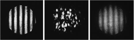
When a spatially modulated light beam is focused with the use of a diffractionlimited optical system with an aperture D > I , two spatially separated light spots are produced in the area of focusing. The optical scheme for such a system is presented in Fig. 4.9. Since two different areas of an object are irradiated, the interaction of these light spots with a scattering medium gives rise to two completely nonidentical (noncorrelated) speckle fields in the diffraction field. If the separation between the interference fringes satisfies the inequality I < dav (the average size of speckles in the observation plane), then the diameter of the beam waist meets the inequality 2w0 > Lφ. In such a situation, regular interference fringes oriented in a random manner from speckle to speckle are observed within the limits of a single speckle. The contrast of fringes depends in this case only on the relation between the intensities of the interfering fields and does not depend on the statistical properties of an object. If I > dav and 2w0 > Lφ, no fringes occur in the scattered field [see Fig. 4.10(b)]. However, when an object moves in the transverse direction, a set of average-intensity interference fringes arises [see Fig. 4.10(c)]. The contrast of this pattern is determined by the statistic properties of the object.
(a) |
(b) |
(c) |
Figure 4.10 Interferograms observed (a) without an object, (b) with a stationary object, and
(c) with a moving object (phantom specklegram).846
The speckle method for testing random phase objects with the use of a spatially modulated beam provides an opportunity to determine such statistical pa-
rameters of an object as the standard deviation σφ and correlation length Lφ of phase fluctuations.343,832,843–846 Strictly speaking, this method can be applied to
phase objects with smooth irregularities and Gaussian statistics. However, this approach can be also employed to study objects with non-Gaussian statistics or sharp inhomogeneities, but calibration is required in this case. Direct measurements using a sufficiently fast detection system make it possible to analyze objects in real time, which is especially important for the investigation of tissue and cellular structures; in particular, in creating optical topographic schemes. This technique can be employed for studying thin layers of human epidermis, thicker transparent tissues of the front segment of the human eye (cornea and crystalline lens), and sclera in
302 |
Coherent Effects in the Interaction of Laser Radiation with Tissues and Cell Flows |
the process of optical clearing (enhanced translucence) under conditions of mechanical or osmotic stresses.172,343,722 Along with the monitoring of statistical pa-
rameters of tissues, this approach should also be useful for the development of the
new generation of laser interferential retinometers, i.e., devices for the determining of retinal visual acuity in the human eye.5,832,847 Since the interference pattern is
statistically averaged as a focused spatially modulated laser beam is scanned, even patients with a turbid (cataractous) crystalline lens can see interference fringes (see Fig. 4.10).
4.4 Dynamic light scattering
4.4.1 Quasi-elastic light scattering
Quasi-elastic scattering of light, photon-correlation spectroscopy, spectroscopy of intensity fluctuations, spectroscopy of intensity fluctuations, and Doppler spectroscopy are synonymous terms related to the dynamic scattering of light, which
underlies a noninvasive method for studying the dynamics of particles on a compar-
atively large time scale.5,78,79,112,113,343,838,
839–841,848,849 The implementation of the single-scattering regime and the use of coherent light sources are of fundamental importance in this case. The spatial scale of testing of a colloid structure (an ensemble of biological particles) is determined by the inverse of the wave vector modulus, |q¯ |−1, defined by Eq. (3.7)
| ¯ | |
|
= |
λ0 |
|
2 |
|
|
q |
−1 |
|
4πn |
sin |
θ |
, |
(4.26) |
|
|
|
where n is the refractive index of the ground substance of the scattering medium (or average refractive index of the ground and scatterer materials, n = n)¯ and θ is the angle of scattering. With allowance for self-beating due to the photomixing of the electric components of the scattered field, we can write the intensity autocorrelation function in the following form:
g2(τ) = I (t)I (t + τ) . |
(4.27) |
For Gaussian statistics, this autocorrelation function is related to the first-order autocorrelation function by the Siegert formula,
g2(τ) = A(1 + βsb|g1(τ)|2), |
(4.28) |
where τ is the delay time; A = i 2 is the square of the mean value of the photocurrent, or the baseline of the autocorrelation function; βsb is the parameter of self-beating efficiency, βsb ≈ 1; and
|
|
|
|
|
E |
(t |
+ |
τ)E(t) |
|
|
g |
1 |
(τ) |
= |
|
|
|
|
(4.29) |
||
|
|E(t)|2 |
|
||||||||
|
|
|
|
|
|
|||||
Tissue Optics: Light Scattering Methods and Instruments for Medical Diagnosis |
303 |
is the normalized autocorrelation function of the optical field. |
|
For a monodispersive system of Brownian particles, we have |
|
g1(τ) = exp(− T τ), |
(4.30) |
where T = q2DT is the relaxation parameter and DT = kBT /6πηrh is the coefficient of translation diffusion, kB is the Boltzmann constant, T is the absolute temperature, η is the absolute viscosity of the medium, and rh is the hydrodynamic radius of a particle. Many biological systems are characterized by a bimodal dis-
tribution of diffusion coefficients, when fast diffusion (DTf) can be separated from slow diffusion (DTs) related to the aggregation of particles.5,849–851 In this case,
the first-order autocorrelation function is written as
g1(τ) = p1 exp&−q2DTsτ' + p2 exp&−q2DTsτ', |
(4.31) |
where p1 and p2 are the coefficients proportional to the concentration and efficiency of scattering of smalland large-sized particles, respectively. The goal of spectroscopy of quasi-elastic scattering is to reconstruct the distribution of scattering particles in sizes, which is necessary for the diagnosis or monitoring of a disease.
4.4.2 Dynamic speckles
The specific features of the diffraction of laser beams from moving phase screens underlie speckle methods of structure diagnostics and monitoring of biological
flows and motion parameters of bioobjects, including biovibrations, which are easy to implement from the technical point of view.22,76,82,83,825–831,833–836,852–858
The fluctuations of individual speckles can be analyzed to provide information about the movement of the scatterers producing the fluctuations. This analysis can be based either on the techniques of photon correlation spectroscopy or laser Doppler velocimetry. It is not intuitively obvious that time-varying speckle and Doppler-induced fluctuations are identical. The theory of time-varying speckle starts with the classical (though random) interference pattern produced when light beams of the same frequency interfere. The fluctuations are caused by the changes in optical path lengths of the interfering beams caused by the movement of the scatterers. Doppler fluctuations, on the other hand, are explained by the beating effect that occurs when two waves of slightly different frequency are superimposed, the difference being due to the frequency shift induced by the Doppler effect when light is scattered by a moving object. Thus, the speckle explanation is based on the superposition of waves of the same optical frequency, whereas in the Doppler explanation the superimposed waves have different frequencies. Despite these apparent differences in approach, it can be shown that mathematically the two expla-
nations lead to identical equations linking the intensity fluctuations to the velocity distribution of the scatterers.82,83 Thus, the two approaches are just different ways
of looking at the same physical phenomenon.
304 |
Coherent Effects in the Interaction of Laser Radiation with Tissues and Cell Flows |
|
In the case of diffraction of a sharply focused Gaussian beam from a moving |
RPS with the Gaussian statistics of phase inhomogeneities and a Gaussian correlation function, the power spectrum of intensity fluctuations in the far-field zone can be represented in the form of homodyne (I) and heterodyne (II) parts as852
S(ω) = C1(2b)0.5 exp − |
b |
ω2 |
I |
|
2 |
+ &C2b0.5 exp,(−b(ω − ω0)2) + exp(−b(ω + ω0)2)-'II . (4.32)
Here, ω = 2πf λ/v is the unscaled frequency; f is the modulation frequency; v is the velocity of a moving RPS,
b = |
Lc2 |
+ 2Mw02 |
, |
|
4M |
and
ω0 = 4πM(w0/Lc)2(x0/z)/(1 + 2M(w0/Lc)2),
where M is the parameter that depends on RPS dispersion of heights (σh) and irradiating wavelength (λ), w0 is the radius of the beam waist, x0 is a fixed point where speckles are observed in the moving frame of reference, and z is the distance between the scattering and observation planes.
For a weakly scattering RPS (e.g., a model of a thin blood vessel), we have M = 1 and C1 C2. For a deep RPS (e.g., a model of a thick blood vessel), we have M (σh/λ)2 and C1 C2. In the case of thin vessels, we should expect the appearance of a high-frequency peak in the spectrum of intensity fluctuations (the heterodyne part of the spectrum) owing to the interference interaction of the specular and scattered components. The specular component (in transmission or reflection) serves as a reference wave. The position of the peak on the frequency scale depends on the observation angle (x0/z). Since the standard deviation of profile fluctuations is small (σh λ), the spectrum S(ω) of intensity fluctuations features only high-frequency components. By contrast, in the model of a deep RPS, because of suppression of the specular component (due to scattering), interference interaction vanishes and the spectrum features only low-frequency components (the homodyne part).
The aforesaid concept is illustrated by theoretical and experimental spectra presented in Figs. 4.11 and 4.12. Thus, the statistical characteristics of transmitted (reflected) light essentially depend on the observation angle and the degree of nonuniformity of an object. Such statistics of speckles are associated with a small number of scatterers and can be classified as statistically nonuniform, non-Gaussian statistics [cf. Eq. (4.18)]. Similar to the case of spectroscopy of quasi-elastic scattering (Doppler spectroscopy), the frequency shift is a linear function of both the velocity

Tissue Optics: Light Scattering Methods and Instruments for Medical Diagnosis |
305 |
Figure 4.11 Normalized theoretical power spectra of intensity fluctuations for dynamic speckles arising from the interaction of a focused laser beam (w0 = 10λ) with phase objects characterized by various degrees of nonuniformity (σh) for different observation angles (x0).852
Figure 4.12 Scattering from a random flow: normalized experimental spectra of fluctuations for dynamic speckles for different observation angles (x0); w0 ≈ 2.3λ; the spectra are averaged over 256 realizations of instantaneous spectra.852
of a scatterer and the observation angle of speckles only when the number of scatterers irradiated by a laser beam is sufficiently large. If the number of scatterers is small, N = (w0/Lc) < 5, we should expect an additional strong dependence of the frequency shift on N in accordance with the theoretical dependence presented in Fig. 4.13.
4.4.3 Full-field speckle technique—LASCA
One problem of using the temporal statistics of time-varying speckle is that measurements are made at only one point in the speckle pattern (a single speckle). If an area needs to be analyzed, it is necessary to scan the detector over the field of view. If a map of velocity distribution is required, some method of scanning the area of interest is necessary. Such a map is of particular importance if blood

306 |
Coherent Effects in the Interaction of Laser Radiation with Tissues and Cell Flows |
Figure 4.13 Normalized theoretical dependence of the central frequency in the spectrum of intensity fluctuations on the number of scatterers, Ns = w0/Lc .852
flow is to be used as a diagnostic tool. A linear CCD array was used to simulta-
neously monitor a line of speckles, and a scanning mirror was used to extend this to a two-dimensional area.859,860 To characterize a local blood flow, the ratio of
the mean intensity to the intensity difference in the speckle pattern was utilized; a quantity called “normalized blur” was a measure of velocity. In particular, a microcirculation map of the retina of a rabbit eye was received while illuminating the retina with light from a diode laser, scanning and storing the speckle images, and then calculating the differences between successive images. These measurements
showed good correlation with invasive methods.860 Scanning has also been applied to the laser Doppler technique,861,862 and commercial scanning Doppler systems
are now on the market that can provide monitoring of capillary blood flow over quite large areas of the body.
However, nonscanning, so-called full-field, techniques for monitoring capillary blood flow are more attractive. The contrast of a speckle pattern used as a measure of time integration of a fluctuating speckle pattern can be employed as a detecting parameter to provide a full-field technique. If the integration time is comparable with the period of the intensity fluctuations caused by dynamic light scattering, it is clear that the effect will be a blurring of the recorded speckle pattern—a reduction in the speckle contrast.
The use of such time-integrated speckle led in the early 1980s to a technique for flow visualization that simultaneously achieves full-field operation and very simple (and cheap) data collection and processing (see Refs. 82, 83, 112, 827, 831, 863, and 865–868). Originally called “single-exposure speckle photography,” it was developed primarily for the measurement of retinal blood flow. The basic technique was simply to photograph the retina under laser illumination using an exposure time that is of the same order as the decorrelation time of the intensity fluctuations. It is clear that a very short exposure time would “freeze” the speckle and result in a high-contrast speckle pattern, whereas a long exposure time would allow the speckles to average out, leading to a low contrast. In general, the velocity distribution in the field of view is mapped as variations in speckle contrast. Subsequent high-pass optical spatial filtering of the resulting photographs converted these contrast variations to more easily seen intensity variations. Later work introduced dig-

308 |
Coherent Effects in the Interaction of Laser Radiation with Tissues and Cell Flows |
and spatial resolution will be lost. In practice, a square of 7 × 7 or 5 × 5 pixels is usually a satisfactory compromise.
As indicated above, the principle of LASCA is very simple. A time-integrated image of a moving object exhibits blurring. In the case of a laser speckle pattern, this appears as a reduction in the speckle contrast, defined (and measured) as the ratio of the standard deviation of the intensity to the mean intensity. This occurs regardless of the “movement” of the speckle. For random velocity distributions, each speckle fluctuates in intensity. For lateral motion of a solid object, on the other hand, the speckles also move laterally and become “smeared” on the image— but a reduction in speckle contrast still occurs. For fluid flow, the situation might be a combination of both these types of “movement.” In each case, the problem for quantitative measurements is the determination of a relationship between the speckle contrast and the velocity (or velocity distribution).
The higher the velocity, the faster are the fluctuations and the more blurring occurs in a given integration time. By making certain assumptions, the following mathematical relationship between the speckle contrast and the temporal statistics of the fluctuating speckle can be found:827
T
σ2s (T ) = 1 g˜2(τ)dτ, (4.33) T
0
where σ2s is the spatial variance of the intensity in the speckle pattern, T is the integration time, g˜2(τ) is the autocovariance of the temporal fluctuations in the intensity of a single speckle, and g˜2(τ) is defined in Eq. (4.20). This equation defines the relationship between LASCA and those techniques that use the intensity fluctuations in laser light scattered from moving objects or particles. LASCA measures the quantity on the left-hand side of Eq. (4.33); photon correlation spectroscopy, laser Doppler, and time-varying speckle techniques measure the quantity on the right-hand side. It is also worth noting that LASCA uses image speckle, whereas most of the temporal techniques use far-field speckle. However, this does not detract from the fundamental equivalence of the two approaches expressed in Eq. (4.33).
All the techniques allow the correlation time τc to be determined. In the case of photon correlation, this parameter is measured directly. In the case of LASCA, some further assumptions must be made in order to link the measurement of speckle contrast with τc.
Depending on the type of motion being monitored, various models can be used to find a relation between the speckle contrast and the correlation time τc for a given integration time T . For example, for the case of a Lorentzian velocity distribution, this relation has a view (see also Fig. 4.15)827
Is |
= |
|
2T |
1 − exp − τc |
|
1/2 |
(4.34) |
. |
|||||||
σ |
|
|
τc |
2T |
|
|
|
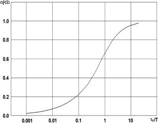
Tissue Optics: Light Scattering Methods and Instruments for Medical Diagnosis |
309 |
Figure 4.15 Variation of speckle contrast with the ratio of decorrelation time (τc) to integration time (T ) for the Lorentzian model of LASCA.827
As all the temporal frequency measurement techniques (photon correlation spectroscopy, laser Doppler, and time-varying speckle), LASCA suffers on the problem of relating the correlation time τc to the velocity distribution of the scatterers. It is not straightforward and depends on the effects of multiple scattering, the size and the shape of the scattering particles, non-Newtonian flow, non-Gaussian statistics, non-Gaussian statistics resulting from a low number of scatterers in the measuring volume, spin of the scatterers, etc. Much work is going on regarding these effects and the question is far from being settled. Because of the uncertainties caused by these factors, it is common in all these techniques to rely mainly on calibration rather than on absolute measurements.
To measure the temporal statistics of fluctuating speckle patterns, it is necessary to monitor the intensity of a single speckle. In order to do this accurately, the aperture of the detector must be smaller than the average speckle size. Otherwise, some spatial averaging will occur and the first-order statistics will be corrupted (some accuracy loss in the second-order statistics may also take place). For LASCA, the matter is more complicated because it computes the local speckle contrast within a square of pixels, the size of the square being under the control of the operator. The larger the square sampled for each measurement the better the statistics. But it is also important to sample a large enough number of speckles as well as pixels: if the speckles are much larger than the pixels, as suggested above, fewer speckles are sampled. This means that the viable speckle size is more restricted. If it is too small, each pixel samples more than one speckle, leading to speckle averaging and loss of measured contrast. If it is too large, not enough speckles are sampled to ensure good statistics. Thus, speckle size needs to be carefully controlled. This can
310 |
Coherent Effects in the Interaction of Laser Radiation with Tissues and Cell Flows |
be done by fixing the aperture of the imaging optics, as this alone determines the speckle size,822 but it removes the control on the amount of light entering the camera, as the shutter speed (the other variable available) has already been determined in order to select the range of velocities to be measured. Unless the dynamic range of the camera is very large, this can be a significant restriction and can require the use of neutral density filters to ensure usable light levels at the detector.
Another problem that has occurred with LASCA is a failure to realize the full range of contrasts that should theoretically be available. A stationary object should give a speckle contrast of unity (σI = I , in accordance with the well-established speckle statistics theory and experiment). A fully blurred speckle pattern produced by rapidly moving scatterers should have zero contrast. The Lorentzian model [see Eq. (4.34) and Fig. 4.15], for example, suggests that for a given integration time T , the dynamic range of the technique that corresponds to contrasts between 0.1 and 0.9 should be about two and a half orders of magnitude in τ (and hence in velocity). In practice, contrasts of only 0.6 were being measured, even for stationary random diffusers.83 One of the possible causes of this is the CCD camera dark current. By carrying out some data preprocessing, it is possible to remove the effect of the dark current and to get the measured speckle contrast for the stationary diffusing surface equal to 0.95, very close to the theoretical value of 1.0 expected for a fully developed speckle pattern.863 Other problems of LASCA connected with the statistics owning to the Gaussian profile of the laser beam and the nonlinearity of the CCD camera also take place.863 However, many of these problems are also characteristic of laser Doppler, photon correlation, and other time-varying speckle techniques.
To summarize, the LASCA technique offers a full-field, real-time, noninva-
sive, and noncontact method of mapping flow fields, such as capillary blood flow.82,83,112,827,831,863,865–868 It uses readily available off-the-shelf equipment and
the software operates in a user-friendly way using the Microsoft Windows NT interface. Laser Doppler, photon correlation spectroscopy, and time-varying speckle are related techniques, but work by analyzing the intensity fluctuations in the scattered laser light. Since they are essentially methods that operate at a single point in the flow field, some form of scanning must be used if a full-field velocity map of the flow area is required. Typical scanning laser Doppler systems take some minutes to complete this scan. LASCA achieves this goal in a single shot by utilizing the spatial statistics of time-integrated speckle. The technique produces a false-color map of blood flow in less than a second, without the need to scan. The main disadvantage of LASCA is the loss of resolution caused by the need to average over a block of pixels in order to produce the spatial statistics used in the analysis. However, the advantage of real-time operation without scanning outweighs the problem of loss of resolution, especially for biomedical applications.
4.4.4 Diffusion wave spectroscopy
Diffusion wave spectroscopy (DWS) is a new class of studies in the field of dynamic light scattering related to the investigation of the dynamics of particles


312 |
Coherent Effects in the Interaction of Laser Radiation with Tissues and Cell Flows |
The quantity s is related to the number of scattering acts N by the relation s = N ls , where ls = (μs)−1. In highly scattering media, e.g., human skin, s can be considered as a statistically independent random walk. The distribution function of photon migration paths p(s) in the medium is determined as the probability that
light will cover the optical paths s, moving from the point r0 to the point rN+1
as869
|
= |
4πsD |
3/2 |
|
| |
4sD |
|2 |
|
|
||
p(s) |
|
|
c |
|
exp |
c |
r0 − rN+1 |
. |
(4.37) |
||
|
|
|
|
|
|
||||||
Here, D is the photon diffusion coefficient [see Eqs. (1.25) and (1.26)], and c is the speed of light in the medium.
The field E(t) interferes with the field E(t + τ) scattered slightly later in the same series of the scattering particles at the instant of time t + τ (see Fig. 4.16). The time it takes the photons to travel the entire optical path in the medium is much shorter than the characteristic time of changing the position of scattering particles in the medium. Thus, as a result of motion of the particles, the phase between fields E(t) and E(t + τ) will be different at different instants of time, or fluctuate. This predetermines temporal fluctuations of the scattered radiation intensity recorded in the far zone. The patterns of the intensity fluctuations (speckles) can be visualized on a screen or sensed by a homodyne detector.872
Quantitatively, these fluctuations are described by the temporal field autocorrelation function
G1(τ) = E (t + τ)E(t) , |
(4.38) |
determined as873
G1(τ) = I0 j 0, |
p(sj ) exp − |
6 |
q2 r2(τ) , |
(4.39) |
$ |
|
N |
|
|
= ∞
where I0 = | E(t)|2 , the angular brackets denote an ensemble average, and q is the change in the wave vectors ki and ki+1,
|
q = |ki − ki+1| = 2k0 sin |
θ |
|
(4.40) |
||
|
|
. |
|
|
||
|
2 |
|
||||
Respectively, |
|
|
|
|
|
|
q2 = 04k02 |
|
|
ls |
|
|
|
(1 − cos θ)1 = 2k0(1 − cos θ ) = 2k0 |
|
, |
(4.41) |
|||
lt |
||||||
where k0 = |ki | = |ki+1|, θ is the angle between the directions ki = ki+1 (i.e., angle of the ith scattering act), and lt is the transport length of the photon free path
Tissue Optics: Light Scattering Methods and Instruments for Medical Diagnosis |
313 |
(which corresponds to the mean distance where a photon completely loses its initial direction of motion) [see Eq. (1.16)].
In an elementary situation where particles move independently of each other, their positions are represented by Gaussian random quantities, and the change in the photon momentum in each scattering event is independent of the position of
a particle; the path-dependent normalized first-order autocorrelation function is written as80
g1(τ, s) = exp − |
4π2 |
r2 |
(τ) |
s |
. |
(4.42) |
3λ2 |
lt |
Here, s is the total photon path length.
In a dense medium, we have s lt. Therefore, in contrast to the case of single scattering, the correlation function g1(τ, s) is sensitive to the motion of a particle on the length scale on the order of λ[s/ lt]−1/2, which is generally much less than λ. Thus, DWS autocorrelation functions decay much faster than analogous functions employed in spectroscopy of quasi-elastic scattering.
Substituting Eq. (4.41) in Eq. (4.39), we find that the normalized temporal field autocorrelation function g1(τ) = G1(τ)/ | E(t)|2 has the form
g1(τ) = |
∞ |
3 k02 |
r |
2(τ) lt ds. |
(4.43) |
|||
p(s) exp − |
||||||||
|
|
1 |
|
|
|
s |
|
|
|
0 |
|
|
|
|
|
|
|
It is seen that, similar to the conventional dynamic light scattering technique,78,79 the change in g1(τ) is determined in terms of their mean-square displacementr2(τ) , with the difference that the slope of g1(τ) increases in proportion to the average number of scattering particles. This has been verified directly by Yodh et al., who used a pulsed laser and gated the broadened response to select photon path lengths of a specific length.874 For continuous wave illumination, Eq. (4.43) is valid given the assumption that the laser coherence length is much longer than the width of the photon path length distribution.
For a system that multiply scatters laser radiation, the transport of the temporal field correlation function is accurately modeled by the correlation diffusion equation,875 i.e.,
&D 2 − cμa − 2cμsDB k02τ'G1(r¯, τ) = −cS(r¯). |
(4.44) |
Here, G1(r,¯ τ) is determined by Eq. (4.38) and is a function of position r¯ and correlation time τ; it has units of energy per area per second; D is the photon diffusion coefficient; k0 is the wave number of the light in the medium; c is the speed of light in the medium; DB ≡ DT = kBT /6πηrh [see Eq. (4.30)]; and S(r¯) is the distribution of light sources with units of photons per volume per second. Note that, similar to μa, describing losses of correlation due to photon absorption, (2μsDB k02τ) is a loss term representing the losing of correlation due to dynamic

314 |
Coherent Effects in the Interaction of Laser Radiation with Tissues and Cell Flows |
processes. The correlation diffusion Eq. (4.44) is valid for turbid samples with the dynamics of scattering particles governed by Brownian motion (DB ). When τ = 0, there is no “dynamical absorption” and Eq. (4.44) reduces to the steadystate photon diffusion equation, described by Eq. (1.17).
The correlation diffusion equation can be modified to account for other dy-
namic processes. In the cases of random flow and shear flow, the correlation diffusion equation becomes876,877
D |
|
2 |
− |
cμ |
a − |
1 |
cμ k2 |
r2 |
(τ) |
− |
|
1 |
cμ k2 |
V 2 |
|
τ2 |
||
|
3 |
3 |
||||||||||||||||
|
|
|
s |
0 |
|
|
s 0 |
|
|
|||||||||
− |
15 cμs−1 eff2 k02τ2 |
G1(r,¯ τ) = −cS(r¯). |
|
(4.45) |
||||||||||||||
|
|
1 |
|
|
|
|
|
|
|
|
|
|
|
|
|
|
|
|
Here, the forth and fifth terms on the left-hand side arise from random and shear flows, respectively, V 2 is the second moment of the particle velocity distribution (assuming the velocity distribution is isotropic and Gaussian), and eff is the effective shear rate. Notice that the “dynamical absorption” for flow in Eq. (4.45) increases with τ2, compared to the τ increase for Brownian motion, because particles in flows travel ballistically; also, DB , V 2 , and eff appear separately because the different dynamical processes are uncorrelated. The form of the “dynamical absorption” term for random flow is related to that for Brownian motion. Both are of the form (1/3)cμsk02 r2(τ) , where r2(τ) is the mean square displacement of
a scattering particle. For Brownian motion, r2(τ) = DB , and for random flow,
r2(τ) = V 2 τ2.
A schematic diagram of a DWS experimental arrangement is presented in Fig. 4.17. It may consist of a multimode optical fiber that transports a laser beam with an adequate coherence length (larger than or equal to the total photon path length s owing to multiple scattering). Laser radiation diffusely scattered within the sample is then collected by means of a single-mode optical fiber, which allows the fluctuations of the light intensity within the coherence area of the scattered radiation to be
Figure 4.17 Schematic diagram of DWS experimental arrangement: 1, laser with a coherence length that is larger or equal to the total photon path length s owing to multiple scattering; 2, fiber optic probe—a multimode irradiating fiber and a single-mode detecting fiber; 3, detecting system—a photomultiplier tube (PMT) or an avalanche photodiode (APD), operated in the photon counting mode and connected with a digital multichannel autocorrelator; 4, blood perfused tissue.

Tissue Optics: Light Scattering Methods and Instruments for Medical Diagnosis |
315 |
recorded by the detecting system; this includes a photomultiplier tube (PMT) or an avalanche photodiode (APD), operated in the photon counting mode and connected with a digital multichannel autocorrelator. The output signal is then processed with an autocorrelator to the temporal intensity correlation function g2(τ) [Eq. (4.27)], which is related to the normalized temporal field autocorrelation function g1(τ) [Eq. (4.29)] by the Siegert relation [Eq. (4.28)]. Further subsequent analysis of the determined g1(τ) can be performed similar to the conventional dynamic light scattering approach, where the autocorrelation function is evaluated by its representation in a semilogarithmic scale.
4.5 Confocal microscopy
Confocal laser scanning microscopy, which employs the confocal principle (with two optically conjugate diaphragms or small-size slits in the object and image
planes) for the selection of scattered photons coming from a given volume (Fig. 4.18), is a well-developed imaging technique for medical investigations.1,3,28,76,120, 122,614,878–898 It is from this technique that the most impressive results on three-
dimensional imaging of living tissues (in particular, skin) have been recently obtained. The resolution of this technique provides an opportunity to recognize different types of cells and simultaneously observe moving blood cells in microvessels.887
Figure 4.18 Principle of confocal microscope.889
In a conventional microscope, the lateral and axial resolutions are not independent. The great advantage of a confocal microscope is that the axial resolu-
tion is enhanced, which results in the “optical sectioning” capability of confocal microscopes.614,878–881 The lateral resolution of a confocal microscope is inversely
proportional to the NA of the microscope objective lens,887
x = |
0.46λ |
(4.46) |
NA . |

316 |
Coherent Effects in the Interaction of Laser Radiation with Tissues and Cell Flows |
The predicted resolution x is 0.4 μm with a 1.2-NA water-immersion objective lens at wavelength λ = 1064 nm. The axial resolution is more sensitive to the numerical aperture of the microscope objective lens. Therefore, to obtain the maximum axial resolution (and, hence, the best degree of optical sectioning), it is preferred to use microscope objectives with the largest numerical aperture. The full width at half-maximum of the axial irradiance distribution defines the axial resolution or optical section thickness,887
z = |
1.4nλ |
(4.47) |
(NA)2 , |
where n is the refractive index of the objective lens immersion medium. The predicted axial resolution z is 1.4 μm with a 1.2-NA water-immersion objective lens at wavelength λ = 1064 nm and n = 1.35. The lateral x and axial z resolution of the confocal microscope measured for the scattering medium with n = 1.35 at λ = 1064 nm for a 1.2-NA objective lens were 0.7 and 3 μm, respectively.887 The differences in predicted and measured resolution can be attributed to spherical aberration. For an oil-immersion microscope objective with a numerical aperture of 1.4 and blue light of wavelength 442 nm, the lateral resolution is 0.14 μm and the axial or depth resolution is 0.23 μm.614
The lateral resolution of a conventional (conv) and a confocal (conf) microscope can be compared.614,880 If the image of a single point specimen is viewed
in reflected light by conventional microscopy, the image intensity distribution is given by
|
2J (r) |
2 |
|
|
Iconv(r)˜ = |
1 |
˜ |
, |
(4.48) |
r |
||||
|
˜ |
|
|
|
where J1 is the first-order Bessel function, r˜ = (2π/λ)(NA)r, and r is the lateral distance in the focal plane. For the confocal case in the presence of the pinhole, the image is now given by
Iconf(r˜) = |
2J1(r) |
|
4 |
(4.49) |
|
r |
˜ |
. |
|||
|
˜ |
|
|
|
|
For the confocal case, the image is sharpened by a factor of 1.4 relative to the conventional microscope. With a confocal microscope, the resolution is about 40% better than in a conventional microscope.
Let us consider axial resolution in a confocal microscope for imaging both points and planes.614,880,881 If a confocal microscope is scanned axially so that
the intensity of light reflected from a plane mirror is detected as a function of the distance that the mirror moves toward the focal plane, the intensity of the reflected light is given by simple paraxial theory as881
|
(υ(z)/2) |
|
2 |
|
Iconf(z) = |
sin |
|
. |
(4.50) |
υ(z)/2 |
Tissue Optics: Light Scattering Methods and Instruments for Medical Diagnosis |
317 |
The symbol υ(z) is a normalized axial coordinate related to the real axial distance z by
υ = 8π nz sin2 α , (4.51)
λ2
where n sin α = NA. At the focal plane, the intensity of the reflected signal is maximal. These equations are valid for the imaging of plane reflectors. For point or line reflectors, Eq. (4.50) becomes
|
(υ(z)/2) |
|
4 |
|
Iconf(z) = |
sin |
|
. |
(4.52) |
υ(z)/2 |
The optical sectioning is weaker for a point or a line than for a plane. All of these equations refer only to bright field imaging in the reflection mode. For fluorescence imaging, which is incoherent light imaging, all of the equations are different.614 Image quality is not only dependent on resolution, but also is very dependent on the contrast of the image.
The principle of the out-of-focal-plane rejection in a confocal microscope is shown in Figs. 4.18 and 4.19. The reflected light from the focal plane passes through the pinhole and reaches the detector. In the case of an unfocused system,
Figure 4.19 Schematic of the confocal probing technique: L1, L2, and L3, short-focus lenses (f = 8 mm) forming in pairs a small-aperture collimator; d1 and d2, limiting diaphragms with diameters of 10 μm; zf , depth of focal point immersion into the medium under study; L, laser source; D, detector of optical radiation; and n0 and n1, refractive indices of the external and studied media.896
318 Coherent Effects in the Interaction of Laser Radiation with Tissues and Cell Flows
the reflected light is spread out over a region larger than the pinhole; only a very small amount of the light from the outside of the focal plane passes the pinhole and is detected. An important problem in confocal microscopy is the optical aberrations that are introduced by the specimen and/or the instrument itself.614
A high image contrast and a high spatial resolution of reflection confocal microscopy (RCM) are achieved due to probing a small (10–100 μm2) volume of the tissue. The localization of a desired signal within the measured volume of such small dimensions becomes possible as a result of mutual optical matching between the laser radiation source, the measured volume, and the photodetector. The field of view of the light source and photodetector are limited by pinholes, which are mounted in the planes of object and image (Fig. 4.19).896 If the penetration depth zf of the lens focus into the tissue does not exceed three to four lengths of the photon mean free path lph [see Eq. (1.8)], then such pinholes ensure that photons reflected strictly back by the tissue and cell components within the probed volume (so-called ballistic photons) dominate in the detected signal. Just these photons carry valid information that allows one to reconstruct the internal structure of the medium under study.
As zf increases, i.e., when the focus penetrates deeper into the scattering medium, the fraction of ballistic photons in the detected signal decreases, while the fraction of photons scattered by the medium increases. Under typical conditions of experiments with biological tissues, RCM allows one to distinguish ballistic photons against a background of the totality of the medium-scattered photons, until zf becomes higher than lph by a factor of 5–8. In other words, because of an intense multiple light scattering characteristic of most of tissues, RCM makes it possible
to obtain an image of the cellular structure of skin, for example, located at a depth of at most 300–400 μm.878,885–887
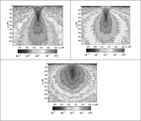
Figure 4.20 shows the results of Monte Carlo simulation of spatial distribution J (r¯) of the probability density of the effective photon optical paths performed for a confocal probing scheme with a focus of the objective lens immersed into a homogeneous scattering medium to a depth of zf = 300 μm. The parameters of RCM are presented in Fig. 4.19. As is expected, when the immersion depth zf does not exceed 3–4 MFPs (μs ≤ 10 mm−1 or, equivalently, lph ≥ 100 μm), clearly pronounced photon focusing at a depth of 300 μm is observed in the spatial distribution of the density of effective optical photon paths [Fig. 4.20(a)].
If zf amounts to 8–20 MFPs (μs = 26.6–40.0 mm−1 and, correspondingly, lph = 25–37.5 μm), then the tendency of probing-radiation focusing in the tissue is still held [Fig. 4.20(b)]. However, the central focal spot region is much larger than in the case of a less scattering medium [Fig. 4.20(a)]. With a further increase in the medium scattering coefficient (μs ≥ 100 mm−1) and the corresponding shortening of photon MFP (lph ≤ 10 μm), the incident radiation turns out to be defocused, although its narrow directivity remains unaltered [Fig. 4.20(c)].
These data (Fig. 4.20) clearly illustrate the possibility of localizing the focused probing laser radiation inside a homogeneous, multiply and anisotropically scattering (g = 0.9) and weakly absorbing (μa = 0.01 mm−1) medium at its probing by RCM.
Tissue Optics: Light Scattering Methods and Instruments for Medical Diagnosis |
319 |
Figure 4.20 Spatial distribution J (r) of the probability density of the effective photon op-
tical |
paths calculated |
for a |
homogeneous |
(n1 = 1.4), multiply [μs = 10 (a), 26.6 (b), |
and |
100 mm−1 (c)], |
and |
anisotropically |
(g = 0.9) scattering, and weakly absorbing |
(μa = 0.01 mm−1) medium at its probing by the reflection confocal microscopy in the geometry presented in Fig. 4.19 and zf = 300 μm.896
4.6 Optical coherence tomography (OCT)
Methods of interferometry and tomography of tissues and organs with the use of partially coherent light sources have progressed rapidly in recent years,1,3,8,17,18,28,
45,76,77,84,102,108–111,116,126,127,129,135,136,138,139,142,343,412–424,620,711–713,716–718,737,
750–753,764–776,899–939 which provided the grounds for organizing a special international conference8,45,116 and special issues of the Journal of Biomedical Optics on this subject.17,18 OCT was first demonstrated in 1991.899 Imaging was performed
in vitro in human retina and in atherosclerotic plaque as examples of imaging in transparent weakly scattering media as well as highly scattering media. A brief
historical review and analysis of the fundamentals of low-coherence interferometry and tomography are presented by Fercher and coworkers,84,142,901,902 who also
discussed ophthalmologic applications of these methods. An overview of the early

320 |
Coherent Effects in the Interaction of Laser Radiation with Tissues and Cell Flows |
development of optical low-coherence reflectometry and some recent biomedical applications is given by Masters.931
Different terms are employed in the literature to specify this method of investigations: dual-beam coherent interferometry or laser Doppler interferometry, optical coherence tomography (OCT) or optical coherence reflectometry. The tomographic scheme differs from the interferometric one by additional transverse scanning, which allows one to obtain topograms of various tissue layers.
OCT is analogous to ultrasonic imaging, which measures the intensity of reflected infrared light rather than reflected sound waves from the sample. Time gating is employed so that the time for the light to be reflected back, or echo delay time, is used to assess the intensity of back-reflection as a function of depth. Unlike ultrasound, the echo time delay on the order of femtoseconds cannot be measured electronically due to the high speed associated with the propagation of light. Therefore, a time-of-flight technique has to be engaged to measure such an ultrashort time delay of light back-reflected from the different depth of a sample. OCT uses an optical interferometer illuminated by a low-coherent-light source to solve this problem.
This technique is conventionally implemented with the use of a dual-beam Michelson interferometer. If the path length of light in the reference arm is changed with a constant linear speed v, then the signal arising from the interference between the light scattered in a backward direction (reflected) from a sample and light in the reference arm is modulated at the Doppler frequency
fD = |
2v |
(4.53) |
λ . |
Owing to the small coherence length of a light source,
lc = |
2 ln(2) λ2 |
(4.54) |
, |
πλ
where λ is the bandwidth of the light source with a Gaussian line profile, the Doppler signal is produced by backscattered light only within a very small region (on the order of the coherence length lc) that corresponds to the current optical path length in the reference arm. If a multimode diode laser or a superluminescent diode (SLD) with a bandwidth of 15–60 nm (λ 800–860 nm) is employed, the longitudinal resolution falls within the range of 5–20 μm. For a titanium sapphire laser
with a wavelength of 820 nm, the bandwidth may reach 140 nm. Correspondingly, the resolution is 2.1 μm.45,84
A typical scheme of a dual-beam Michelson interferometer with a lowcoherence source and the principle of operation of such a device are shown in Fig. 4.21, which illustrates ophthalmologic applications of this technique.901,902 Let us consider the interference of light reflected from the front surface of eye cornea
(1) and pigment epithelium of retina (2). Under these conditions, each of the two beams E and E is split into two beams, E1, E2 and E1 , E2 . Suppose that d is
Tissue Optics: Light Scattering Methods and Instruments for Medical Diagnosis |
321 |
Figure 4.21 Dual-beam Michelson interferometer with a partially coherent source of excitation for ophthalmologic applications:901,902 SLD, superluminescent diode; M and M , interferometer mirrors; DB, dual beam; and PD, photodetector.
the geometric distance between the reflective surfaces of the eye. Then, the components of the field are characterized by additional delay times and the total field of light beams reflected from the eye is written as
E(t) = E1(t)+ E2(t − τ) = E1(t)+ E1 (t − δ)+ E2(t − τ)+ E2 (t − δ − τ), (4.55)
where τ = 2nd/c0 and n is the refractive index of a medium between two reflective surfaces. When quasi-monochromatic sources are used, the interfering beams consist of groups of waves, and n should be replaced by the group refractive index
dn |
|
ng = n − λ dλ . |
(4.56) |
We should take into account that the coherence length of light increases in a dispersive medium, and spatial resolution lowers. This is especially noticeable for broadband laser systems. Specifically, for a titanium sapphire laser with a band-
width of 140 nm, the coherence length is equal to 2.1 μm for air (in the absence of dispersion) and 60 μm for water (in a layer with a thickness of 24 mm).917
According to Ref. 917, the coherence length in a medium is
lc = |
lc2 + |
2 |
|
1/2 |
(4.57) |
|
dλ d λ |
, |
|||||
|
|
|
dng |
|
|
|
where d is the thickness of the medium. Hence, we find that if the thickness of a tissue being probed is not large (on the order of 1 mm), the additive to the coherence length due to dispersion may remain small. For example, for a titanium sapphire laser with the largest bandwidth, this addition is the same order of magnitude as the coherence length in free space.

322 |
Coherent Effects in the Interaction of Laser Radiation with Tissues and Cell Flows |
Figure 4.22 presents a typical waveform of the interference signal corresponding to in vivo probing of the fundus of the human eye with the use of partially coherent beams of the interferometer shown schematically in Fig. 4.21. By analyzing such a signal, one can very accurately determine the thickness of the layer of nerve fibers (the distance between ILM and GCL, 75 μm). Along with geometric parameters, partially coherent interferometry provides an opportunity to determine optical parameters of tissues, such as scattering and absorption coefficients and the refractive index. The dependence of these parameters on the physiological state of a tissue allows one to obtain reliable diagnostic data in both ophthalmology and other fields of medicine. It was demonstrated that the spatial resolution of the interference technique is approximately an order of magnitude higher than the spatial resolution provided by conventionally employed ultrasonic diagnosis. In addition, owing to its contactless character, the interference technique does not require eye anesthesia. The results of measurements obtained with the use of the interference
technique are characterized by a high reproducibility and can be easily interpreted, even by nonexperts.901,902 In addition to the determination of geometric and optical
parameters of the rear segment of the human eye (the thickness of the fundus and its components), low-coherence interferometry can be successfully used to measure the thickness of the cornea with a resolution on the order of 1.6–3.5 μm, which is necessary for monitoring during conventional and laser surgical operations aimed at changing the refraction of the cornea; for assessing various corneal pathologies, including edema; and for measuring the depth of the front eye chamber and the axial length of an eye. The latter possibility is especially important when cataracts are
treated surgically, because an error of 0.2–0.3 mm in determining the axial length of an eye gives rise to an error in eye refraction of about one diopter.901,902
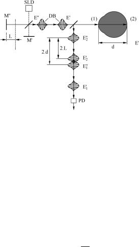
OCT can also be described on the basis of the principles of the heterodyne technique.939 Figure 4.23 shows a typical fiber-optical scheme, where two beams
Figure 4.22 Interference signal (in arbitrary units) obtained by in vivo probing of the fundus of the human eye. The wavelength of the radiation of a superluminescent diode is 825 nm, and its coherence length is 12 μm901,902; ILM, inner boundary layer; GCL, ganglion layer; RPE, retinal pigment epithelium; and CH1 and CH2, choroid layers. The distance is measured relative to the cornea.

Tissue Optics: Light Scattering Methods and Instruments for Medical Diagnosis |
323 |
Figure 4.23 A typical fiber-optic OCT system. Light from the superluminescent diode (SLD) is split up by a beam splitter into a local oscillator (LO) beam and a signal beam that is incident on to the medium (tissue) under investigation. The reflected field is superposed with the LO beam reflected from the longitudinally scanned reference mirror; the superposed field is measured by a detecting-demodulating system.939
(signal and local oscillator beam) are generated from a broadband source such as an SLD. The signal beam is incident on the sample; the transmitted or scattered light is then superposed with the local oscillator beam in the balanced detector. Due to the broad spectrum of the light (and, therefore, small longitudinal coherence length), the light coming from the sample and the local oscillator beam only interfere if their path lengths are matched within the coherence length of the light. By increasing the path length of the local oscillator beam l with the reference mirror MR , the local oscillator beam interferes only with those parts of the signal field that have traveled the same distance l in the medium. Therefore, signal field contributions from different photon path lengths in the sample can be selected. In practice, the reference mirror is moved at a fixed speed, and the heterodyne beat signal resulting from the Doppler shift of the local oscillator beam reflected from the moving mirror is recorded at the same time [see Eq. (4.53)]. By moving the laser beam in a twodimensional raster and taking vertical scans for each point, a three-dimensional image can be obtained.
Figure 4.24(a) shows an example of a time-modulated interference signal detected by the photodetector. If the detected ac signal is band-pass filtered with respect to the central Doppler frequency (as the center frequency) it is then rectified and low-pass filtered. The output of the low-pass filter is the envelope of the time-modulated ac interference signal, which is equivalent to the cross-correlation amplitude. Figure 4.24(b) gives an example of the detected envelope corresponding to Fig. 4.24(a).
OCT performs cross-sectional imaging by measuring the time delay and magnitude of optical echoes at different transverse positions, essentially by the use

324 |
Coherent Effects in the Interaction of Laser Radiation with Tissues and Cell Flows |
(a)
(b)
Figure 4.24 Low-coherence interferometer output signals: (a) time-modulated ac term of interference signal, (b) corresponding signal after demodulation (cross-correlation amplitude, i.e., envelope).932
of low-coherence interferometry. A cross-sectional image is acquired by performing successive rapid axial measurements while transversely scanning the incident sample beam onto the sample (see Fig. 4.25). The result is a two-dimensional data set, which represents the optical reflection or backscattering strength in a crosssectional plane through a biological tissue. The system implemented by the opticfiber couplers, matured in the telecommunication industry, offers the greatest advantage for the OCT imaging of biological tissues because it can be integrated
into almost all the currently available medical imaging modalities, for example, endoscope and microscope.108,109,111,717,775 Figure 4.23 gives an example of the
fiber-optic versions of OCT.
Numerous fiber-optical OCT systems are described in the literature (see, for example, Refs. 1, 108, 109, 111, 127, 136, and 142). In these systems, light from a low-coherence light source is coupled to a single-mode fiber coupler where half of the light power is conducted through the single-mode fiber to the reference mirror. The remaining half enters the sample via proper focusing optics. The distal end of the fiber in the sample arm serves a dual role as a coherent light receiver
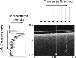
Tissue Optics: Light Scattering Methods and Instruments for Medical Diagnosis |
325 |
Figure 4.25 OCT image (right-hand lower) is generated by performing measurements of the reflected signal time delay and magnitude of backscattered light intensity (left) over a range of transverse positions (upper). As an example, the OCT image of a ceramic material with glazing that models a hard tissue (tooth or bone) is presented.932
and spatial filter analogous to a confocal pinhole. Because the dc signal and intensity noise generated by the light from the reference arm add to the interference signal, it makes the system prone to excess photon noise. One way to reduce this type of noise is to use a balanced detection configuration that would cancel the
background noise components by subtracting the photocurrents generated by two photodetectors.932,939 The interference signals at the output of the detectors add
because they vary out of phase.
OCT has the advantage that it can achieve extremely high axial image resolution independently of the transverse image resolution. The axial resolution is determined by the coherence length of light source used, i.e., Eq. (4.54), which is independent of the sampling beam focusing conditions. The lateral or transverse resolution achieved with an OCT imaging system is determined by the focused spot size limited by the numerical aperture of the lens used to deliver the light onto the sample, and the wavelength, as in conventional or confocal microscopy [see Eqs. (4.48) and (4.49)].
4.7 Second-harmonic generation
Second-harmonic generation (SHG) is a new high-resolution nonlinear optical imaging modality for study of intact tissues and cellular membranes.940–948 SHG
is a second-order nonlinear optical process that can only arise from media lacking a center of symmetry, e.g., an anisotropic crystal or at an interface such as
membrane. It can be used to image highly ordered structural proteins without any exogenous labels,940,941,943–948 as well as biological membrane probes with high
membrane specificity.942
Collagen as a main component of connective tissues has an appreciable nonlinear susceptibility for SHG.940,941,943–948 The helix of the collagen secondary struc-
ture is noncentrosymmetric, satisfying a condition for SHG, which self-assembles

326 |
Coherent Effects in the Interaction of Laser Radiation with Tissues and Cell Flows |
into higher-order structures. Collagen has been shown to have a dominant uniaxial second-order nonlinear susceptibility component aligned along the fiber axis. In such multicomponent tissues as skin, SHG light is generated mostly within dermis, not in cellular layers like epidermis or subcutaneous fat. The SHG technique has a number of advantages connected with the incident wavelength dividing and selectivity to tissue structure, which allow one to easily reject surface reflection and multiple scattering of the incident light in the epidermis layer without any gating technique. In addition, SHG polarimetry is an effective tool to probe collagen orientation in tissues.944–947
In general, the nonlinear polarization for a material can be expressed as942
P = |
|
+ |
|
+ |
|
+ · · · |
|
|
|
χ(1)E |
|
χ(2)EE |
|
χ(3)EEE |
|
, |
(4.58) |
where P is the induced polarization, χ(n) is the nth order nonlinear susceptibility,
and is the electric field vector of the incident light. The first term describes
E
normal absorption and reflection of light; the second, SHG, sum, and difference frequency generation; and the third, both twoand three-photon absorption, as well as third-harmonic generation.
SHG, by contrast to two-photon fluorescence (see Section 1.7.2), does not arise from an absorptive process. Instead, an intense laser field induces a nonlinear second-order polarization in the assembly of molecules, resulting in the production of a coherent wave at exactly twice the incident frequency (or half the wavelength). The spectral and temporal profiles of two-photon excited fluorescence and SHG are also different. For two-photon fluorescence, the width of the emission spectrum is determined by the relative geometries of the ground and excited molecular state, and the emission lifetime is related to the oscillator strength of the transition and is typically on the order of a few nanoseconds. In SHG, by contrast, both the spectral and temporal√ characteristics are derived from the laser source: the bandwidth scales as 1/ 2 of the bandwidth of the excitation laser and, due to the coherence of the process, the SHG pulse is temporally synchronous with the excitation pulse.
A simplified expression for the SHG signal intensity has the form942
I (2ω) χ(2) |
E(ω) |
|
2 |
(4.59) |
|
τp, |
|||
τp |
where χ(2) is the second-order nonlinear susceptibility, and E(ω) and τp are the laser pulse energy and width, respectively. As in two-photon fluorescence [see Eq. (1.189)], the signal is quadratic with peak power, but since SHG is an instantaneous process, a signal is generated only during the duration of the laser pulse. The macroscopic value χ(2) can be expressed in terms of the first molecular hyperpolarizability β as
χ(2) = ρM β , |
(4.60) |
Tissue Optics: Light Scattering Methods and Instruments for Medical Diagnosis |
327 |
where ρM is the density of molecules and the brackets denote an orientational average. This underscores the need for a noncentrosymmetric region, since β would vanish for an isotropic distribution of dipole moments. As it follows from Eqs. (4.59) and (4.60), the SHG signal depends on the square of the molecular surface density, whereas two-photon fluorescence intensity is linear with the density of fluorophores [see Eq. (1.189)].
Within the two-level system model, the first molecular hyperpolarizability β is given by942
β = |
3e2 |
|
|
ωgefge μge |
, |
(4.61) |
2h3 |
|
[ωge2 |
− ω2][ωge2 − 4ω2] |
|||
|
¯ |
|
|
|
|
|
where e is electron charge, ωge, fge, and μge are the energy difference, oscillator strength, and change in dipole moment between the ground and excited states, respectively. While SHG is not an absorptive process, the magnitude of the SHG wave can be resonance enhanced when the energy of the second-harmonic signal overlaps with an electronic absorption band. It follows from Eq. (4.61) that β becomes large when the laser fundamental frequency approaches the electronic transition, and then the total second-order response is a sum of the nonresonant and resonant contributions,
χtotal(2) = χnonres(2) + χres(2). |
(4.62) |
Depending on the specific properties of the molecule and the excitation wavelength, the resonant contribution can dominate, resulting in enhancement of an order of magnitude or more.