

5. Non-relativistic quantum mechanics
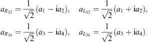
The above discussed transformation of the Kepler problem can now be used to calculate the energy levels of the hydrogen atom as was described in [15]. To this purpose one introduces holomorphic coordinates
|
|
(5.1) |
so that the Hamiltonian H4 in (4.19) can be written as:
|
|
(5.2) |

where k = e2. Introducing then holomorphic coordinates for left and right moving quanta
|
|
(5.3) |
the Hamiltonian (5.2) turns into
|
|
(5.4) |
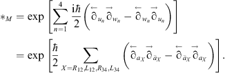
One can now quantize this system with the Moyal product. The four-dimensional Moyal star product transforms under KS-transformation and the above transformations into
|
|
(5.5) |
The
energy levels can then be obtained by the
![]() -genvalue
equation
-genvalue
equation
|
|
(5.6) |
where
![]() is
the product of four Wigner functions of the one-dimensional harmonic
oscillator given in (2.6).
Eq.
(5.6)
gives then
is
the product of four Wigner functions of the one-dimensional harmonic
oscillator given in (2.6).
Eq.
(5.6)
gives then
|
e2= |
(5.7) |
To get the energy levels of the hydrogen atom one has to impose the constraint
|
|
(5.8) |
which
for the energy levels corresponds to nR12-nL12+nR34-nL34=0
or nR12+nR34=nL12+nL34≡n-1.
Putting this and
![]() into
(5.7)
one gets the well-known energy levels of the hydrogen atom
into
(5.7)
one gets the well-known energy levels of the hydrogen atom
|
|
(5.9) |
Geometric algebra in a fermionic star product formulation can be used in general to describe quantum mechanics, when combined in a straightforward way with the bosonic star product formalism. In classical mechanics described with geometric algebra and the Clifford star product the fermionic part of the underlying superanalysis was deformed and the basis vectors played only a mathematical role by generating the structures of vector analysis. Going over to quantum mechanics means that also the scalar coefficients of superanalysis have to be multiplied by a deformed product, namely the bosonic Moyal star product. This leads then to a deformed version of geometric algebra and describing geometric algebra in terms of star products allows to combine the Clifford star product and the Moyal product into one star product, which should be called Moyal–Clifford product. The Clifford product on the phase space that described the structures of classical Hamilton mechanics was given by (4.20). In quantum mechanics one needs now a product with which general multivector functions on the phase space are multiplied. These multivector functions are the observables of the theory and as such can only be multivectors in the space basis vectors σr. So one has to go over from the Clifford product (4.20) to the Clifford product (3.14), which can be done by implementing constraints that identify the corresponding basis vectors [6]. The Moyal–Clifford product for a single particle system is then
|
|
(5.10) |

To see the consequences of the additional Moyal deformation in geometric algebra one can for example consider the Moyal–Clifford product of two vectors in d = 2 dimensions. The generalization of (3.15) can be written as
|
a |
(5.11) |
Under
the Moyal product the coefficients in general do not commute if they
are functions of qn
and pn.
This means that the Moyal–Clifford product of the same vectors
a![]() MCa
is in general not a scalar, but has also a bivector part. It is this
additional bivector part, which appears only for
MCa
is in general not a scalar, but has also a bivector part. It is this
additional bivector part, which appears only for ![]() ≠0,
that constitutes the spin as a physical observable. This can be seen
if one considers the minimal substituted Hamiltonian which is in the
formalism of deformed geometric algebra given by:
≠0,
that constitutes the spin as a physical observable. This can be seen
if one considers the minimal substituted Hamiltonian which is in the
formalism of deformed geometric algebra given by:
|
|
(5.12) |
|
|
(5.13) |
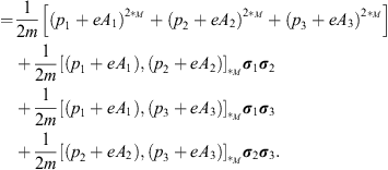
The
first three terms
![]() describe
the Landau problem of a charged particle in a magnetic field which
can be solved in the star product formalism as described in [16]
or [7].
The other three terms that describe the interaction of the spin and
the magnetic field appear only because of the Moyal product. If the
magnetic field points in σ3-direction
the vector potential is given by
describe
the Landau problem of a charged particle in a magnetic field which
can be solved in the star product formalism as described in [16]
or [7].
The other three terms that describe the interaction of the spin and
the magnetic field appear only because of the Moyal product. If the
magnetic field points in σ3-direction
the vector potential is given by
![]() and
only the first Moyal-commutator contributes:
and
only the first Moyal-commutator contributes:
|
|
(5.14) |
where
![]() and
σ3=-iσ1σ2
is a real quaternion, which is constructed according to Figs. (3.13)
and (2.14).
The difference between this calculation and the conventional approach
is that in the conventional formalism the Clifford structure is
introduced by putting in Pauli matrices by hand in (5.12).
The Pauli matrices describe the spin and lead analogously to the
additional term HS,
this is known as the Feynman trick [17].
In geometric algebra the Clifford structures do not have to be added,
they are just the basis vectors that already exist in classical
mechanics, but become apparent as physical objects in the quantum
case. It is then straightforward to calculate the
and
σ3=-iσ1σ2
is a real quaternion, which is constructed according to Figs. (3.13)
and (2.14).
The difference between this calculation and the conventional approach
is that in the conventional formalism the Clifford structure is
introduced by putting in Pauli matrices by hand in (5.12).
The Pauli matrices describe the spin and lead analogously to the
additional term HS,
this is known as the Feynman trick [17].
In geometric algebra the Clifford structures do not have to be added,
they are just the basis vectors that already exist in classical
mechanics, but become apparent as physical objects in the quantum
case. It is then straightforward to calculate the
![]() -eigenfunctions
of HS
which turn out to be the spin Wigner functions described in Section 1
[7].
-eigenfunctions
of HS
which turn out to be the spin Wigner functions described in Section 1
[7].
One
should note that the Moyal–Clifford product is a product for
functions on the phase space, which play the role of observables. As
seen above these observables are in general multivectors, where the
terms of higher grade are described by the space basis vectors σn
and not by the phase space basis vectors ηn
and ρn,
because the latter are not observable quantities. Nevertheless the
basis vectors of phase space can be considered to play an indirect
role in the expression (2.1)
of the Moyal product, because the imaginary structure
![]() can
be interpreted as a two blade on phase space. If the phase space is
just two dimensional there is only one candidate for the imaginary
structure, namely the symplectic volume form j = ηρ.
That the i
in the Moyal product has to be an unit area bivector can be seen from
the integral representation of the Moyal product [18]:
can
be interpreted as a two blade on phase space. If the phase space is
just two dimensional there is only one candidate for the imaginary
structure, namely the symplectic volume form j = ηρ.
That the i
in the Moyal product has to be an unit area bivector can be seen from
the integral representation of the Moyal product [18]:
|
|
(5.15) |
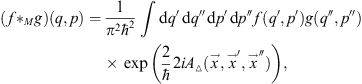
where
![]() is
the area of the triangle spanned by the vectors
is
the area of the triangle spanned by the vectors
![]() ,
,
![]() and
and
![]() .
So i
plays here the role of the unit area bivector in phase space. The
two-dimensional Moyal product can then be written with the gradient
.
So i
plays here the role of the unit area bivector in phase space. The
two-dimensional Moyal product can then be written with the gradient
![]() x = η∂q + ρ∂p
as:
x = η∂q + ρ∂p
as:
|
|
(5.16) |
so that the correspondence principle has the form
|
|
(5.17) |
One should also note the similarity to the fermionic star product of two vectors a = a1η + a2ρ and b = b1η + b2ρ:
|
|
(5.18) |
where
A![]() (a, b)
is the area of the triangle spanned by the vectors a
and b.
(a, b)
is the area of the triangle spanned by the vectors a
and b.