2. The star product formalism

We first want to introduce the star product formalism in bosonic and fermionic physics with the example of the harmonic oscillator [5]. The bosonic oscillator with the Hamilton function , can be quantized by using the Moyal product

(2.1)

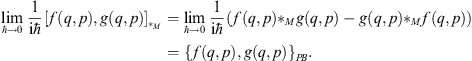
The star product replaces the conventional product between functions on the phase space and it is so constructed that the star anticommutator, i.e., the antisymmetric part of first order, is the Poisson bracket:

(2.2)

This relation is the principle of correspondence. The states of the quantized harmonic oscillator are described by the Wigner functions . The Wigner functions and the energy levels E_n of the harmonic oscillator can be calculated with the help of the star exponential

(2.3)

where Hⁿ_M=H_M…_MH is the n-fold star product of H. The star exponential fulfills the analogue of the time dependent Schrödinger equation

(2.4)

The energy levels and the Wigner functions fulfill the -genvalue equation

(2.5)

and for the harmonic oscillator one obtains and

(2.6)

where the L_n are the Laguerre polynomials. The Wigner functions are normalized according to and the expectation value of a phase space function f can be calculated as

(2.7)

The same procedure can now be used for the grassmannian case [6]. The simplest system in grassmannian mechanics [8] is a two-dimensional system with Lagrange function

(2.8)

With the canonical momentum

(2.9)

the Hamilton function is given by

(2.10)

Together with Eq. (2.9) this Hamiltonian suggests that the fermionic oscillator describes rotation. Indeed, calculating the fermionic angular momentum, which corresponds to the spin, leads to

S3=θ1ρ2-θ2ρ1=-iθ1θ2,

(2.11)

so that the Hamiltonian in (2.10) can also be written as H = ωS₃. As a vector the angular momentum points out of the θ₁-θ₂-plane. Therefore, we consider the two-dimensional fermionic oscillator as embedded into a three-dimensional fermionic space with coordinates θ₁, θ₂, and θ₃. Note that we choose both for the fermionic space and momentum coordinates the units .

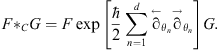
Quantizing the fermionic oscillator [6] involves a star product that is given by

(2.12)

We will call this star product the Clifford star product because it leads to a cliffordization of the Grassmann algebra of the θ_i. This can be seen by considering the star-anticommutator that is given by

{θi,θj}C=θiCθj+θjCθi=δij.

(2.13)

Since the Grassmann variables

(2.14)

fulfill the relations

(2.15)

with [σⁱ,σ^j]_C=σⁱ_Cσ^j-σ^j_Cσⁱ, they correspond to the Pauli matrices. From equations Figs. (2.11) and (2.14) it follows that and . Note that {1, σ¹, σ², σ³} is a basis of the even subalgebra of the Grassmann algebra and that this space is also closed under _C multiplication.

In the space of Grassmann variables there exists an analogue of complex conjugation, which is called the involution. As in [8] it can be defined as a mapping , satisfying the conditions

(2.16)

where c is a complex number and its complex conjugate. For the generators θ_i of the Grassmann algebra we assume , so that for σⁱ defined in (2.14) the relation holds true. This corresponds to the fact that the 2 × 2 Pauli matrices are hermitian.

We now define the Hodge dual for Grassmann numbers with respect to the metric δ_ij. The Hodge dual maps a Grassmann monomial of grade r into a monomial of grade d−r, where d is the number of Grassmann basis elements (which is in our case three):

(2.17)

With the help of the Hodge dual one can define a trace as

(2.18)

The integration is given by the Berezin integral for which we have ∫dθ_iθ_j=δ_ij, where the on the right-hand side is due to the fact that the variables θ_i have units of . The only monomial with a non-zero trace is 1, so that by the linearity of the integral we obtain the trace rules

(2.19)

With the fermionic star product (2.12) one can—as in the bosonic case—calculate the energy levels and the -eigenfunctions of the fermionic oscillator. This can be done with the fermionic star exponential

(2.20)

where the Wigner functions are given by

(2.21)

The fulfill the -genvalue equation for the energy levels . The Wigner functions are complete, idempotent and normalized with respect to the trace, i.e., they fulfill the equations

(2.22)

respectively. Furthermore, they correspond to spin up and spin down states since (2.21) corresponds to the spin projectors and the expectation values of the angular momentum are

(2.23)

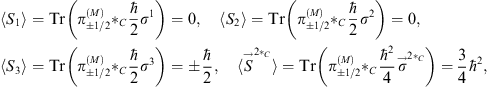
where the spin was used with components of as defined in (2.14).

In the fermionic θ-space the spin is the generator of rotations, which are described by the star exponential

(2.24)

where we used the definition with rotation angle and a rotation axis given by the unit vector . The vector transforms passively according to

(2.25)

with being the well-known SO (3) rotation matrix. The axial vector transforms in the same way. Note that the passive transformation (2.25) of the θ_i amounts to an active transformation of the components x_i in the vector .