4. Equation for particle trajectories

The equation of motion of fine particles in a fluid with an acoustic sound field is given from Eq. (7). In the literature, the inertia term x″ is neglected because it is small and the singular perturbation solution shown in Eq. (8) is used.

Using Eq. (8) forces the initial velocity to be k/c sin βx₀ (it is usually assumed = 0) and leads to errors in the solution that for very small time t, can be as large as k/c. The solution obtained by using the approximation equation (8) with initial value x(0) = x₀ can easily be obtained:

(29)

By separation of variables:

(29)

(30)

(31)

To obtain a more accurate approximation than the singular perturbation solution, let the assumed solution of Eq. (7) be of the form:

x=u+xs.

(32)

Substituting Eq. (32) in Eq. (7), one obtains:

(33)

Assuming that u is small, it follows from Eq. (30) that the terms in brackets above are small, and it is reasonable to approximate u by solving the following initial value problem:

(34)

Here it is assumed that x′(0) = v(0) = 0 in Eq. (7). The solution of Eq. (34) can be readily found by elementary means to be:

(35)

(36)

where,

(37)

(38)

and r₁ >>>r₂. It is therefore plausible that the following approximate solutions (t) are quite accurate for all t:

(39)

(40)

In fact, it can be proved rigorously that

(41)

and

(42)

Note also then that:

(43)

Therefore, particle trajectories in the acoustic medium can be calculated using Eq. (39) with the given values of constants (c, k, β). In graph Fig. 6, the vertical axis represents the time in seconds for the sound field treatment. The values on the horizontal axis represent the position of particles at corresponding times. The distances are in micrometers and for convenience taken at λ/16 of wavelength intervals from the first pressure anti-node at the face of the transducer. All the particles move toward the pressure node to which the particles are supposed to move. Particles with 2 μm diameter take about 20 s to reach the node. Fig. 5 shows where the sinks (pressure nodes) repeat at every 2π/β distance. Thus the behavior of the particle movement shown in Fig. 6 using the trajectory equation represents the actual behavior of the system.

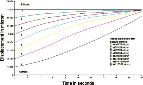
Fig. 6. Particle trajectories.

5. Concentration equation

The approximate solution of Eq. (39), obtained earlier will be used to obtain an approximate value of the particle concentrations. Since the particles are neither created nor disappear during the irradiation of sound, the equation of conservation of particles must hold:

(44)

In order to use this equation, one must find an expression for the velocity field v = v(x, t) as a function of just x and t. Now if the singular perturbation approximation v  v_s = k/c sinβx_s is used, one can simply substitute v(x, t) = v_s(x, t) = v_s(x) = k/c sinβx_s in Eq. (44), with x_s a function of t and x₀, and get the result in the literature. A more accurate solution is obtained by employing the approximate formula of Eq. (39):

(45)

for the solution of Eq. (7) subject to the initial conditions x(0) = x₀, x′(0) = 0. In order to do this one must find the velocity of the particle at distance x from the pressure anti-node at time t > 0, so that one can find the approximation for v as a function of x and t.

To use the approximation equation (45) for the determination of the particle concentration, one must extract from it an approximation for v(x, t) to be substituted into Eq. (44), hence one must first solve:

(46)

Let the solution of the above equation for x₀ in terms of x and t be denoted by x₀ = ψ(x, t). This cannot be done in closed form, but the following can readily be shown, by solving Eq. (30) for x₀, to yield a good approximate solution for all 0 < x < π/β, t > 0:

(47)

From the above equation one can obtain a good approximation for the velocity field to be used in Eq. (44) by replacing x₀ with ψ in Eq. (40):

(48)

where n is the velocity at a given x and t. Substituting the value of ψ from Eq. (47) into Eq. (48), and using the fact that r₁  r₂, yields the approximation:

(49)

As e^−βkt/c  1 for all except very large t, Eq. (49) yields:

(50)

an even simpler approximation for v:

Hence,

(51)

Observe that converges very rapidly to v_s(x) = k/csinβx with increasing t. Substituting for v in Eq. (44), one obtains:

(52)

which must be solved subject to the initial condition (Cauchy problem):

n(x,0)=n0(const).

(53)

Therefore, the following approximation formula for the concentration is applicable for any time t:

(54)

Observe that this is very close to the formula:

(55)

obtained using the singular perturbation approximation, except for t very close to zero. For 0 < t  1, the difference between Eq. (54) and the above (55) formula can be O(10¹). It is worth noting in closing that it can be shown by a long and tedious-but straightforward-computation that the error in using Eq. (54) is  2βk/c, for all 0  x  π/β, t  0.

The ratio of the initial concentration (n₀) to final concentration (n) at that time (t), is taken as 1 when time = 0. Using Eq. (54) the particle concentrations with increasing t values are given on graph in Fig. 7 represent the concentration at different times; note how the concentrations are highest at the sink π/β (Fig. 5). Thus one sees that the approximate concentration closely follows the behavior of the actual system.

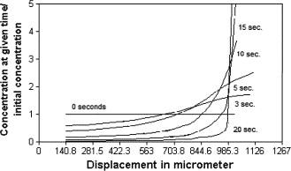
Fig. 7. Particle concentration.

The approximate solutions for particle trajectories and concentration will be used to compare the experimental observations with expected theoretical values. There is no closed form solution for Eq. (7), and direct application of a Runge–Kutta solver led to rather surprising results that were completely unsatisfactory. Stiff ODE solvers also appeared somewhat inadequate, so a viable approach was to use an approximate solution. If the experimental results can be compared to Fig. 6 and Fig. 7, then it can be stated that the mathematical model derived has solutions that are in good agreement with the actual behavior of the system and can quite possibly be generalized for any type of medium or particle.