

4. Asymmetric quartic double-well problem
The
hierarchy theorem established in the previous section has two
restrictions: (i) the limitation of half-space x ![]() 0
and (ii) the requirement of a monotonically decreasing perturbative
potential w (x).
In this section, we shall remove these two restrictions.
0
and (ii) the requirement of a monotonically decreasing perturbative
potential w (x).
In this section, we shall remove these two restrictions.
Consider the specific example of an asymmetric quadratic double-well potential
|
|
(4.1) |
with the constant λ > 0. The ground state wave function ψ (x) and energy E satisfy the Schroedinger equation
|
(T+V(x))ψ(x)=Eψ(x), |
(4.2) |
where
![]() ,
as before. In the following, we shall present our method in two
steps: We first construct a trial function
,
as before. In the following, we shall present our method in two
steps: We first construct a trial function
![]() (x)
of the form
(x)
of the form
|
|
(4.3) |
At
x = 0,
![]() (x)
and
(x)
and
![]() ′ (x)
are both continuous, given by
′ (x)
are both continuous, given by
|
|
(4.4) |
and
|
|
(4.5) |
with
prime denoting
![]() ,
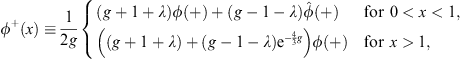
as before. As we shall see, for x > 0,
the trial function
,
as before. As we shall see, for x > 0,
the trial function
![]() (x) =
(x) = ![]() + (x)
satisfies
+ (x)
satisfies
|
|
(4.6a) |
with
|
|
(4.7a) |
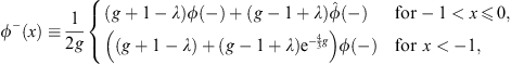
whereas
for x < 0,
![]() (x) =
(x) = ![]() − (x)
satisfies
− (x)
satisfies
|
|
(4.6b) |
with
|
|
(4.7b) |
Furthermore, at x = ±∞
|
v+(∞)=v-(-∞)=0. |
(4.8) |
Starting
separately from
![]() + (x)
and
+ (x)
and
![]() − (x)
and applying the hierarchy theorem, as we shall show, we can
construct from
− (x)
and applying the hierarchy theorem, as we shall show, we can
construct from
![]() (x)
another trial function
(x)
another trial function
|
|
(4.9) |
with χ (x) and χ′ (x) both continuous at x = 0, given by
|
χ(0)=χ+(0)=χ-(0) |
(4.10) |
and
|
χ′(0)=χ+′(0)=χ-′(0)=0. |
(4.11) |
In addition, they satisfy the following Schroedinger equations
|
|
(4.12) |
and
|
|
(4.13) |
From V (x) given by (4.1) with λ positive, we see that at any x > 0, V (x) > V (−x); therefore, E+ > E−.
Our second step is to regard χ (x) as a new trial function, which satisfies
|
(T+V(x)+w(x))χ(x)=E0χ(x) |
(4.14) |
with w (x) being a step function,
|
|
(4.15) |
and
|
|
(4.16) |
We see that w (x) is now monotonic, with
|
w′(x) |
(4.17) |
for the entire range of x from −∞ to +∞. The hierarchy theorem can be applied again, and that will lead from χ (x) to ψ (x), as we shall see.
4.1. Construction of the first trial function
We consider first the positive x region. Following Section 2.1, we begin with the usual perturbative power series expansion for
|
ψ(x)=e-gS(x) |
(4.18) |
with
|
gS(x)=gS0(+)+S1(+)+g-1S2(+)+ |
(4.19) |
and
|
E=gE0(+)+E1(+)+g-1E2(+)+ |
(4.20) |
in which Sn (+) and En (+) are g-independent. Substituting Figs. (4.18), (4.19) and (4.20) into the Schroedinger equation (4.2) and equating both sides, we find
|
|
(4.21) |
|
|
(4.22) |
etc. Thus, (4.21) leads to
|
|
(4.23) |
Since the left side of (4.22) vanishes at x = 1, so is the right side; hence, we determine
|
E0(+)=1+λ, |
(4.24) |
which leads to
|
S1(+)=(1+λ)ln(1+x). |
(4.25) |
Of course, the power series expansion Figs. (4.19) and (4.20) are both divergent. However, if we retain the first two terms in (4.19), the function
|
|
(4.26) |
serves
as a reasonable approximation of ψ (x)
for x > 0,
except when x
is near zero. By
differentiating
![]() (+),
we find
(+),
we find
![]() (+)
satisfies
(+)
satisfies
|
(T+V(x)+u+(x)) |
(4.27) |
where
|
|
(4.28) |
In
order to construct the trial function
![]() (x)
that satisfies the boundary condition (4.5),
we introduce for x
(x)
that satisfies the boundary condition (4.5),
we introduce for x ![]() 0,
0,
|
|
(4.29) |
and
|
|
(4.30) |
so
that
![]() + (x)
and its derivative
+ (x)
and its derivative
![]() +′ (x)
are both continuous at x = 1,
and in addition, at x = 0
we have
+′ (x)
are both continuous at x = 1,
and in addition, at x = 0
we have
![]() +′ (0) = 0.
For
x
+′ (0) = 0.
For
x ![]() 0,
we observe thatV (x)
is invariant under
0,
we observe thatV (x)
is invariant under
|
|
(4.31) |
The
same transformation converts
![]() + (x)
for x
positive to
+ (x)
for x
positive to
![]() − (x)
for x
negative. Define
− (x)
for x
negative. Define
|
|
(4.32) |
where
|
|
(4.33) |
|
|
(4.34) |
and
|
|
(4.35) |
Both
![]() − (x)
and its derivative
− (x)
and its derivative
![]() −′ (x)
are continuous at x = −1;
furthermore,
−′ (x)
are continuous at x = −1;
furthermore,
![]() + (x)
and
+ (x)
and
![]() − (x)
also satisfy the continuity condition Figs. (4.4)
and (4.5),
as well as the Schroedinger equation Figs. (4.6a)
and (4.6b),
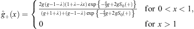
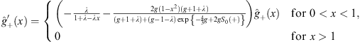
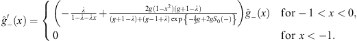
with the perturbative potentials v+ (x)
and v- (x)
given by
− (x)
also satisfy the continuity condition Figs. (4.4)
and (4.5),
as well as the Schroedinger equation Figs. (4.6a)
and (4.6b),
with the perturbative potentials v+ (x)
and v- (x)
given by
|
|
(4.36a) |
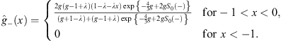
and
|
|
(4.36b) |
in which u+ (x) is given by (4.28),
|
|
(4.37) |
|
|
(4.38a) |
and
|
|
(4.38b) |
In
order that u+ (x),
![]() be
positive for x > 0
and u- (x),
be
positive for x > 0
and u- (x),
![]() positive
for x < 0,
we impose
positive
for x < 0,
we impose
|
|
(4.39) |
in addition to the earlier condition λ > 0. From Figs. (4.28) and (4.37), we have
|
|
(4.40a) |
and
|
|
(4.40b) |
Likewise, from Figs. (4.38a) and (4.38b), we find
|
|
(4.41a) |
and
|
|
(4.41b) |
Furthermore, as x → ±1,
|
|
(4.42a) |
and
|
|
(4.42b) |
Thus,
for x ![]() 0,
we have
0,
we have
|
|
(4.43) |
and, together with Figs. (4.36a) and (4.40a),
|
|
(4.44a) |
for
x
positive. On the other hand for x ![]() 0,
0,
![]() is
not always positive; e.g., at x = 0,
is
not always positive; e.g., at x = 0,
|
|
which
is positive for
![]() ,
but at x = −1+,
,
but at x = −1+,
|
|
However,
at x = −1,
![]() .
It is easy to see that the sum
.
It is easy to see that the sum
![]() can
satisfy for x
can
satisfy for x ![]() 0,
0,
|
|
(4.44b) |
To
summarize:
![]() + (x)
and
+ (x)
and
![]() − (x)
satisfy the Schroedinger equation Figs. (4.6a)
and (4.6b),
with v± (x)
given by Figs. (4.36a)
and (4.36b),
− (x)
satisfy the Schroedinger equation Figs. (4.6a)
and (4.6b),
with v± (x)
given by Figs. (4.36a)
and (4.36b),
|
|
(4.45a) |
and
|
|
(4.45b) |
and the boundary conditions Figs. (4.4) and (4.5). In addition, v± (x) satisfies
|
|
(4.46) |
and the monotonicity conditions Figs. (4.7a) and (4.7b).