2. Application of Newton’s second law

The proposed technology can be implemented in a rectangular narrow channel of upward fluid flow. Two walls of the channel can be made with a piezoelectric transducer and rigid reflecting surface, as shown in Fig. 2. When the transducer is energized at the proper frequency to maintain a resonant acoustic field, there will be a pressure node located on the mid-plane of the chamber, and pressure antinodes located on the chamber walls. The acoustic force on a suspended particle results from the particle–fluid interaction that arises when the particle and suspending fluid have different acoustic properties. When the particle is at the pressure node at quarter wavelength, mid-plane of the chamber width, the magnitude of this force is the maximum. For a dilute suspension, the secondary radiation forces, the body forces and the hydrodynamic interactions are neglected. The rate of change of particle momentum is equal to:

(ρpV0+0.5ρfV0)dv/dt=FPARF+FPTRF+V0(ρp-ρf)g+FD,

(3)

mva=FPARF+FPTRF+V0(ρp-ρf)g+FD,

(4)

where v is the particle velocity and g is the gravitational acceleration. The mass in the momentum term is the “virtual mass” of the particle, m. Since the particle’s velocity is v, the drag force is given by Stokes’ law (F_D = −6πμrv), where μ is the viscosity of the fluid and r is the radius of the particle in suspension. The summation of the forces in the direction of the acoustic wave propagation gives:

Fac=FPARF=mva+6πμrv=V0EackGsin(2kx).

(5)

Thus the acoustic force, F_ac, on a particle in an acoustic field is due to the primary axial radiation force and can be used to calculate the particle trajectories.

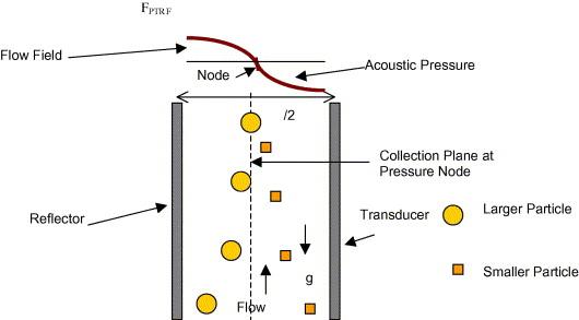
Fig. 2. Schematic showing the mechanics of the proposed technology.

3. Mathematical model

In this research fractionation of particles is based on density and compressibility differences of fluid and particles rather than on particle size. Employing the above basic principles of physics of particles in an acoustic field, a mathematical model is developed to calculate trajectories of deflected particles subjected to acoustic standing waves. Table 1 gives the properties of the particles and the fluid that are used in this research.

Table 1.

Properties of particles and suspending medium

Description	Solid (SiC)	Medium (DI water)
Density (ρ) (kg/m3)	3217	1000
Frequency of sound in medium (f) (kHz)	–	333
Viscosity of medium (μ) (N s/μm2)	–	9.98E−16
Acoustic energy in medium (J/m3)	–	133
Power in medium (W/m3)	–	56 000
Quality factor (Q) of chamber	–	5000

Rearranging Eqs. Figs. (3) and (5) yields the following equation:

(6)

Simplifying Eq. (6) with values in Table 1 yields:

x″+cx′-ksinβx=0,

(7)

where

x′=ν,

(8)

where, c = 1.42E6, k = E8, and β = 2.78E−3 are constants representing the physical parameters of Eq. (7). This equation will be constantly used during the mathematical derivation. The notation (′) indicates the derivative, d/dt, and x is the position of the migrating particle in the x-direction between a transducer and a reflector separated by one half wavelength (=λ/2) of the resonant sound at the given frequency. The parameters c, k, and β are all positive constants having the following orders (O) of magnitude: c = O(10⁶), k = O(10⁸), β = O(10⁻³).

A study of the behavior of the solutions is discussed with an explanation of the available solution techniques. Solutions of Eq. (7) will be used as a basis for concluding some results during the derivation. The above equation is extremely stiff, so most numerical solution methods—even stiff equation solvers—provide little useful information.

Note that Eq. (7) has the form somewhat like a damped nonlinear spring (or pendulum) equation. Several publications cited in the literature assumed instantaneous viscous relaxation where the inertial term dv/dt or x″ was neglected. This type of singular perturbation approximation; namely:

cx′-ksinβx=0

(9)

has been used to approximate the solution for Eq. (7). It will be shown in this paper that although this approximation produces results that are qualitatively correct, quantitative errors are incurred that can be significant for some applications.