3.5.2. Restriction

It is also interesting to work out how the local scale transforms in going from a_t to ã_t. A measure of this is . A similar calculation starting from (22) gives, in the same limit as above

(24)

Now something special happens when κ = 8/3. The drift term in d (h′ (a_t)) does not then vanish, but if we take the appropriate power it does. This implies that the mean of is conserved. Now at t = 0 it takes the value , where Φ_A = h₀ is the map that removes A. If K_t hits A at time T it can be seen from (22) that . On the other hand, if it never hits A then . Therefore, gives the probability that the curve γ does not intersect A.

This is a remarkable result in that it depends only on the value of at the starting point of the SLE (assuming of course that Φ_A is correctly normalised at infinity). However, it has the following even more interesting consequence. Let . Consider the ensemble of all SLE_8/3 in H, and the sub-ensemble consisting of all those curves γ which do not hit A. Then the measure on the image in H is again given by SLE_8/3. The way to show this is to realise that the measure on γ is characterised by the probability P (γ ∩ A′ = ) that γ does not hit A′ for all possible A′. The probability that does not hit A′, given that γ does not hit A, is the ratio of the probabilities and P (γ ∩ A = ). 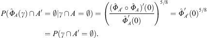By the above result, the first factor is the derivative at the origin of the map which removes A then A′, while the second is the derivative of the map which removes A. Thus

(25)

Since this is true for all A′, it follows that the law of given that γ does not intersect A is the same as that of γ. This is called the restriction property. Note that while, according to Property 3.2, the law of an SLE in any simply connected subset of H is determined by the conformal mapping of this subset to H, the restriction property is stronger than this, and it holds only when κ = 8/3.

We expect such a property to hold for the continuum limit of self-avoiding walks, assuming it exists. On the lattice, every walk of the same length is counted with the same weight. That is, the measure is uniform. If we consider the sub-ensemble of such walks which avoid a region A, the measure on the remainder should still be uniform. This will be true if the restriction property holds. This supports the identification of self-avoiding walks with SLE_8/3.

3.6. Radial sle and the winding angle

So far we have discussed a version of SLE that gives a conformally invariant measure on curves which connect two distinct boundary points of a simply connected domain . For this reason it is called chordal SLE. There are variants which describe other situations. For example, one could consider curves γ which connect a given point r₁ on the boundary to an interior point r₂. The Riemann mapping theorem allows us to map conformally onto another simple connected domain, with r₂ being mapped to any preassigned interior point. It is simplest to choose for the standard domain the unit disc U, with r₂ being mapped to the origin. So we are considering curves γ which connect a given point e^iθ₀ on the boundary with the origin. As before, we may consider growing the curve dynamically. Let K_t be the hull of that portion which exists up to time t. Then there exists a conformal mapping g_t which takes UK_t to U, such that g_t (0) = 0. There is one more free parameter, which corresponds to a global rotation: we use this to impose the condition that is real and positive. One can then show that, as the curve grows, this quantity is monotonically increasing, and we can use this to reparametrise time so that . This normalised mapping then takes the growing tip τ_t to a point e^iθ_t on the boundary.

Loewner’s theorem tells us that , when expressed as a function of g_t (z), should be holomorphic in apart from a simple pole at e^iθ_t. Since g_t preserves the unit circle outside should be pure imaginary when |g_t (z)| = 1, and in order that , it should approach 1 as g_t (z) → 0. The only possibility is

(26)

This is the radial Loewner equation. In fact this is the version considered by Löewner [4].

It can now be argued, as before, that given lk and lk (suitably reworded to cover the case when r₂ is an interior point) together with reflection, θ_t must be proportional to a standard Brownian motion. This defines radial SLE. It is not immediately obvious how the radial and chordal versions are related. However, it can be shown that, if the trace of radial SLE hits the boundary of the unit disc at e^iθ_t1 at time t₁, then the law of K_t in radial SLE, for t < t₁, is the same chordal SLE conditioned to begin at e^iθ(0) and end at e^iθ_t1, up to a reparametrisation of time. This assures us that, in using the chordal and radial versions with the same κ, we are describing the same physical problem.

However, one feature that the trace of radial SLE possesses which chordal SLE does not is the property that it can wind around the origin. The winding angle at time t is simply θ_t − θ₀. Therefore, it is normally distributed with variance κt. At this point we can make a connection to the Coulomb gas analysis of the O (n) model in Section 2.4.1, where it was shown that the variance in the winding angle on a cylinder of length L is asymptotically (4/g)L. A semi-infinite cylinder, parametrised by w, is conformally equivalent to the unit disc by the mapping z = e^−w. Asymptotically, Re w → Re w − t under Loewner evolution. Thus, we can identify L t and hence

κ=4/g.

(27)