5.4. Differential equations

In this section, we discuss how the linear second order differential equations for various observables which arise from the stochastic aspect of SLE follow equivalently from the null state condition in CFT. In this context they are known as the BPZ equations [33]. As an example consider Schramm’s formula (30) for the probability P that a point ζ lies to the right of γ, or equivalently the expectation value of the indicator function which is 1 if this is satisfied and zero otherwise. In SLE, this expectation value is with respect to the measure on curves which connect the point a₀ to infinity. In CFT, as explained above, we can only consider curves which intersect some -neighbourhood on the real axis. Therefore P should be written as a ratio of expectation values with respect to the CFT measure

(58)

We can derive differential equations for the correlators in the numerator and denominator by inserting into each of them a factor (1/(2πi)∫_Γα (z)T (z) dz + c.c., where α (z) = 2/(z−a₀), and Γ is a small semicircle surrounding a₀. This is equivalent to making the infinitesimal transformation z → z + 2/(z − a₀). As before, the c.c. term is equivalent to extending the contour in the first term to a full circle. The effect of this insertion may be evaluated in two ways: by shrinking the contour onto a₀ and using the OPE between T and _2,1 we get

(59)

while wrapping it about ζ (in a clockwise sense) we get

(60)

The effect on _2,1 (r₂) vanishes in the limit r₂ → ∞. As a result we can ignore the variation of the denominator in this case. Equating Figs. (59) and (60) inside the correlation function in the numerator then leads to the differential equation (29) for P found in Section 4.1.

5.4.1. Calogero–Sutherland model

While many of the results of SLE may be re-derived in CFT with less rigour but perhaps greater simplicity, the latter contains much more information which is not immediately apparent from the SLE perspective. For example, one may consider correlation functions _1,2 (r₁)_1,2 (r₂)  _2,1 (r_N)   of multiple boundary condition changing operators with other operators either in the bulk or on the boundary. Evaluating the effect of an insertion (1/2πi)∫_Γ T (z) dz/(z − r_j) where Γ surrounds r_j leads to a second order differential equation satisfied by the correlation function for each j.

This property is very powerful in the radial version. Consider the correlation function

CΦ(θ1,…,θN)=2,1(θ1)2,1(θN)Φ(0)

(61)

of N_2,1 operators on the boundary of the unit disc with a single bulk operator Φ at the origin. Consider the effect of inserting (1/2πi)∫_Γ α_j (z)T (z) dz, where (cf. (26))

(62)

and Γ surrounds the origin. Once again, this may be evaluated in two ways: by taking Γ up to the boundary, with exception of small semicircles around the points e^iθ_k, we get G_jC_Φ, where G_j is the second order differential operator

(63)

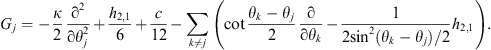
The first three terms come from evaluating the contour integral near e^iθ_j, where α_j acts like (the term comes from the curvature of the boundary), and the term with k ≠ j from the contour near e^iθ_k, where it acts like .

On the other hand, shrinking the contour down on the origin we see that α_j (z) = z + O (z²), so that on Φ (0) it has the effect of , where the omitted terms involve the L_n and with n > 0. Assuming that Φ is primary, these other terms vanish, leaving simply . Equating the two evaluations we find the differential equation

GjCΦ=xΦCΦ.

(64)

In general there is an (N − 1)-dimensional space of independent differential operators G_j with a common eigenfunction C_Φ. (There is one fewer dimension because they all commute with the total angular momentum ∑_j(∂/∂θ_j).) For the case N = 2, setting θ = θ₂ − θ₁, we recognise the differential operator in Section 4.3.3.

In general these operators are not self-adjoint and their spectrum is difficult to analyse. However, if we form the equally weighted linear combination , the terms with a single derivative may be written in the form ∑_k(∂V/∂θ_k) (∂/∂θ_k) where V is a potential function. In this case it is well known from the theory of the Fokker–Plank equation that G is related by a similarity transformation to a self-adjoint operator. In fact [36] if we form |Ψ_N|^2/κG|Ψ_N|^−2/κ, where Ψ_N=∏_j<k(e^iθ_j-e^θ_k) is the ‘free-fermion’ wave function on the circle, the result is, up to calculable constants the well-known N-particle Calogero–Sutherland hamiltonian

(65)

with β = 8/κ. It follows that the scaling dimensions of bulk operators like Φ are simply related to eigenvalues Λ_N of H_N by

(66)

where . Similarly C_Φ is proportional to the corresponding eigenfunction. In fact the ground state (with conventional boundary conditions) turns out to correspond to the bulk N-leg operator discussed in Section 2.4.2. The corresponding correlator is |Ψ_N|^2/κ.