

3.1. Preliminary analysis
There is no closed form solution for Eq. (7), so one has to rely on qualitative and approximate analysis techniques that will be discussed in this section. Useful information on the nature of the solutions of Eq. (7) can be obtained by recasting it as a two-dimensional system and performing a careful phase plane analysis. To do this, first set x′ = ν and then rewrite (7) as the following system in the x, ν-plane:
|
ν′=ksinβx-cν |
(10) |
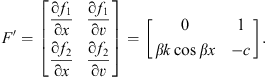
Eq. (10) in matrix form, with f1 and f2 as function of x′ and v′ respectively is:
|
|
(11) |
The
fixed (critical or stationary) points of Eq. (11)
are those points in the x,
ν-plane
satisfying function F(x,ν)=0![]() ν=0,
ksinβx-cν=0:
ν=0,
ksinβx-cν=0:
|
|
(12) |
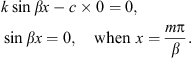
Hence, these points are (mπ/β, 0), where m is an integer. To find the local behavior of the solutions to Eq. (11) near the fixed points, the derivative of F, F′, is computed at these fixed points:
|
|
(13) |
Consequently,
when
![]() ,
and when m
is even:
,
and when m
is even:
|
|
(14) |
and when m is odd:
|
|
(15) |
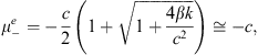
To compute the spectral properties of Eqs. Figs. (14) and (15), one needs to calculate the eigenvalues of the derivative matrices. The eigenvalues (μ) of Eq. (14) are the roots of the equation:
|
|
(16) |
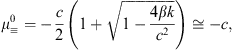
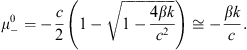
Hence,
there is one negative eigenvalue (![]() )
and one positive eigenvalue (
)
and one positive eigenvalue (![]() )
given, respectively, by
)
given, respectively, by
|
|
(17) |
|
|
(18) |
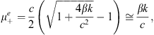
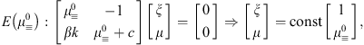
where the approximate formulas follow from Eq. (7). The eigenspaces (E) associated to these eigenvalues are calculated as follows:
|
|
(19) |
|
|
(20) |
Similarly, the eigenvalues of Eq. (15) are the roots of the equation:
|
|
(21) |
Both
of these roots are negative. One of these
![]() has
a large magnitude and the other
has
a large magnitude and the other
![]() has
small absolute value; these are given as:
has
small absolute value; these are given as:
|
|
(22) |
|
|
(23) |
The corresponding eigenspaces (E) are:
|
|
(24) |
|
|
(25) |

It
is concluded that the fixed points of the form (2lπ/β, 0)
are all saddle points having local phase plane behavior as shown in
Fig.
3,
where l
is any integer
![]() 0.
Note that the angle θ
between eigenvector (wu)
and x axis is
0.
Note that the angle θ
between eigenvector (wu)
and x axis is
![]() .
.
![]()
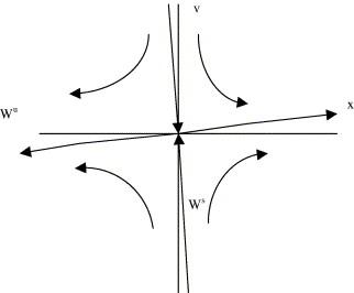
Fig. 3. Phase plane near (2lπ/β, 0).
![]()
On the other hand, the fixed points of the form ((2l + 1)π/β, 0) are all sinks with local phase plane behavior shown below in Fig. 4. Fig. 5 shows the entire phase plane of Eq. (11) obtained by collecting the above results.
![]()
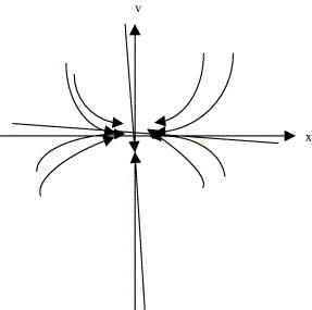
Fig. 4. Phase plane near ((2l + 1)π/β, 0).
![]()
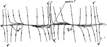
Fig. 5. Phase portrait of Eq. (11).
![]()
Useful
information on the solutions of Eq. (7)
(and equivalently (11))
can be extracted from the above analysis. The relevant portion of the
phase plane for our research is the region R = {(x, v):0 ![]() x
x ![]() 8π/β}.
Clearly any trajectory θt(x0, v0) = (x(t), v(t))
starting at (x0, v0)
8π/β}.
Clearly any trajectory θt(x0, v0) = (x(t), v(t))
starting at (x0, v0) ![]() R,
except for points on the stable manifold, has the property:
R,
except for points on the stable manifold, has the property:
|
|
(26) |
Moreover,
|
|
(27) |
In
fact, all of these trajectories converge very rapidly to the
separatrix G![]() (which is just the portion of the unstable manifold for the origin,
(which is just the portion of the unstable manifold for the origin,
![]() ,
that is contained in R).
This separatrix appears to be quite close to the graph of v = k/c
sinβx,
and so one can infer the following result that shall be proved in the
sequel:
,
that is contained in R).
This separatrix appears to be quite close to the graph of v = k/c
sinβx,
and so one can infer the following result that shall be proved in the
sequel:
|
|
(28) |
One
can also see from the above analysis that the often-used singular
perturbation approximation Eq. (8)
is not really adequate to represent the solutions of Eq. (7)
(![]() (11)).
This is because it is just a single curve in the phase plane region R
beginning at origin, O = (0, 0),
and terminating at (π/β, 0);
albeit a curve to which (almost) all of the solutions (trajectories,
orbits) of Eq. (7)
converge to rather rapidly as t → ∞(x → π/β).
(11)).
This is because it is just a single curve in the phase plane region R
beginning at origin, O = (0, 0),
and terminating at (π/β, 0);
albeit a curve to which (almost) all of the solutions (trajectories,
orbits) of Eq. (7)
converge to rather rapidly as t → ∞(x → π/β).
Since
Eq. (7)
(![]() (11))
has no closed form solution, it is natural to try to compute
numerical approximate solutions using a standard ODE solver such as
the Runge–Kutta method. However, an attempt to apply the
Runge–Kutta method to Eq. (7)
directly leads to rather surprising results that are completely
unsatisfactory. To explain what happens, first note that the system
form of Eq. (7),
namely (11),
is such that there is an enormous discrepancy between the magnitude
of the derivative of the first component f1: = v
and the corresponding magnitudes of the second component
f2:=ksinβx-cv;
in fact, the ratios of the second set of magnitudes to the first is
at least O(108).
Such systems of differential equations are called stiff. In the
presence of such enormous magnitudes, one might expect to encounter
some problems with conventional ordinary differential equation (ODE)
solvers. More specifically, in order to obtain good accuracy using
the Runge–Kutta method one should take a time step of size (h),
no more than about h = 0.1
in order to benefit from the global approximation error of O(h4)
of the Runge–Kutta method. If one uses this increment, it is found
that there is a little movement in the trajectory after several
hundred steps, so if one starts in R
near x = 0,
very little progress is made in moving across R
to the point (π/β, 0)
even after hundreds of steps. Furthermore, if one continues this for
thousands of steps, round-off errors accumulate to the point where
the approximate numerical solution starts behaving in ways that are
not consistent with the properties of the solution that are deduced
from the above analysis.
(11))
has no closed form solution, it is natural to try to compute
numerical approximate solutions using a standard ODE solver such as
the Runge–Kutta method. However, an attempt to apply the
Runge–Kutta method to Eq. (7)
directly leads to rather surprising results that are completely
unsatisfactory. To explain what happens, first note that the system
form of Eq. (7),
namely (11),
is such that there is an enormous discrepancy between the magnitude
of the derivative of the first component f1: = v
and the corresponding magnitudes of the second component
f2:=ksinβx-cv;
in fact, the ratios of the second set of magnitudes to the first is
at least O(108).
Such systems of differential equations are called stiff. In the
presence of such enormous magnitudes, one might expect to encounter
some problems with conventional ordinary differential equation (ODE)
solvers. More specifically, in order to obtain good accuracy using
the Runge–Kutta method one should take a time step of size (h),
no more than about h = 0.1
in order to benefit from the global approximation error of O(h4)
of the Runge–Kutta method. If one uses this increment, it is found
that there is a little movement in the trajectory after several
hundred steps, so if one starts in R
near x = 0,
very little progress is made in moving across R
to the point (π/β, 0)
even after hundreds of steps. Furthermore, if one continues this for
thousands of steps, round-off errors accumulate to the point where
the approximate numerical solution starts behaving in ways that are
not consistent with the properties of the solution that are deduced
from the above analysis.
In
conclusion, the properties of the solutions of Eq. (7)
(![]() (11))
discussed above actually reveal the source of the problems
encountered using numerical methods. Suppose the trajectory starts at
a point (x0, v0)
in R
near (0, 0). Then this trajectory converges to the separatrix Γ
very rapidly, in fact, the distance between θt(x0, v0)
and Γ
decreases with time as e−ct.
Once θt
is very close to Γ
(which is
(11))
discussed above actually reveal the source of the problems
encountered using numerical methods. Suppose the trajectory starts at
a point (x0, v0)
in R
near (0, 0). Then this trajectory converges to the separatrix Γ
very rapidly, in fact, the distance between θt(x0, v0)
and Γ
decreases with time as e−ct.
Once θt
is very close to Γ
(which is
![]() ),
it moves towards R
near (π/β, 0)
as eβkt/c.
Hence, the time required to get very close to (π/β,
0) is roughly eβkt/c=π/β
),
it moves towards R
near (π/β, 0)
as eβkt/c.
Hence, the time required to get very close to (π/β,
0) is roughly eβkt/c=π/β![]() t=c/βk
log (π/β),
thus it follows from the orders of magnitude of the constants
(c, k, β)
that the time required is roughly O(102).
So with a time step of about h = 0.1,
the number of steps required to come close to seeing the asymptotic
nature of the solution as t → ∞
is O(103).
Using this many steps is not only computationally expensive; it also
makes the contamination of the approximate numerical data by round
off errors almost inevitable. Moreover, one can see from the
intrinsic nature of the solutions described above that the basic
problems with numerical solutions cannot be ameliorated through the
use of standard rescaling techniques, nor can they completely
circumvented using the usual stiff equation solvers. One infers from
all of this that we shall need to employ other methods to determine
useful approximate trajectories of Eq. (7)
that stretch all the way from an initial point (x0, v0)
to a very small neighborhood of the sink (π/β, 0)
and that these methods must be of an asymptotic nature for t → ∞.
t=c/βk
log (π/β),
thus it follows from the orders of magnitude of the constants
(c, k, β)
that the time required is roughly O(102).
So with a time step of about h = 0.1,
the number of steps required to come close to seeing the asymptotic
nature of the solution as t → ∞
is O(103).
Using this many steps is not only computationally expensive; it also
makes the contamination of the approximate numerical data by round
off errors almost inevitable. Moreover, one can see from the
intrinsic nature of the solutions described above that the basic
problems with numerical solutions cannot be ameliorated through the
use of standard rescaling techniques, nor can they completely
circumvented using the usual stiff equation solvers. One infers from
all of this that we shall need to employ other methods to determine
useful approximate trajectories of Eq. (7)
that stretch all the way from an initial point (x0, v0)
to a very small neighborhood of the sink (π/β, 0)
and that these methods must be of an asymptotic nature for t → ∞.