

Understanding the Human Machine - A Primer for Bioengineering - Max E. Valentinuzzi
.pdf48 |
Understanding the Human Machine |
Two basic variables in the cardiovascular system (see above) are pressure and flow, respectively analogous to voltage and current. Both are periodic and mathematically unknown functions of time t. However, they are not sinusoidal. Figure 2.14 displays aortic pressure (upper channel), picked up by a miniature transducer placed almost at the root of the vessel with a catheter inserted via a femoral artery, and aortic flow (lower channel), detected by means of an electromagnetic flowmeter embracing the artery after the arch. The animal was an anesthetized dog. The foot of each beat in the pressure record (diastolic pressure) marks the opening of the aortic valve, hence, ejection starts, and the record below shows a rapid upstroke. The indentation after the maximum value (systolic pressure) marks the closure of the same valve. It is called the dicrotic notch, DN, a handy flag present in any good quality arterial pressure record. As a consequence, flow drops to zero after having shown a maximum. The two vertical bars clearly bound ejection time, ET, which in this particular case is in the order of 300 ms.
After having obtained experimental digital records of pressure, P = p(t), and of flow, F = q(t), they are subjected to spectral analysis, usually by means of the Fast Fourier Transform (FFT). The latter algorithm is readily available in many commercial softwares, for which the student should be familiar with Fourier series to better understand it. In other words, each signal is decomposed in its dc (Po, Qo), and sinusoidal components (pn, qn), in which the fundamental frequency, f1, coincides with the heart rate, HR. Thus,
ET
Figure 2.14. AORTIC PRESSURE (upper curve) AND AORTIC FLOW (lower curve). Experimental time course records from which the aortic input impedance can be calculated as explained in the text. The dicrotic notch in the upper channel marks the end of ejection. ET = ejection time, between the opening and the closure of the aortic valve. Obtained from an experimental dog at the Department of Bioengineering, UNT, 1994.
Chapter 2. Source: Physiological Systems and Levels |
49 |
|
p(t)= Po + p1 |
+ p2 +K+ pn |
(2.32) |
q(t)= Qo + q1 |
+ q2 +K+ qn |
(2.33) |
where pn = Pn cos (nωt+θn) and qn = Qn cos (nωt+ψn). Phases or angles are represented by θn and ψn. In practice, it is enough to keep up to the tenth harmonic (n = 10), as it is well documented in the literature (Geddes, 1970).
It is now the time to calculate the impedance, both in modulus and in angle, for each harmonic component by extension of the definition used in electrical circuits:
Zo = Ro = Po Qo |
(2.34) |
Zl = Pl / Ql |
(2.35) |
M
Zn = Pn / Qn (2.36)
for the moduli, and 0 and φn = θn – ψn , for the phases. Observe that the dc component of the arterial impedance component has a zero angle (thus, pressure and flow are in phase) and its modulus Zo coincides with its real part Ro, which, in turn, coincides with the peripheral resistance Rp, introduced earlier above. Obviously, the hydraulic input arterial impedance concept is more general than the simpler Poiseuille’s definition,
min/l] |
160 |
|
|
|
|
|
|
|
|
|
|
|
|
|
|
|
|
140 |
|
|
|
|
|
|
|
|
|
|
|
|
|
|
|
||
[mmHg |
|
|
|
|
|
|
|
|
|
|
|
|
|
|
|
||
120 |
|
|
|
|
|
|
|
|
|
|
|
|
|
|
|
||
100 |
|
|
|
|
|
|
|
|
|
|
|
|
|
|
|
||
Impedance |
80 |
|
|
|
|
|
|
|
|
|
|
|
|
|
|
|
|
60 |
|
|
|
|
|
|
|
|
|
|
|
|
|
|
|
||
40 |
|
|
|
|
|
|
|
|
|
|
|
|
|
|
|
||
20 |
|
|
|
|
|
|
|
|
|
|
|
|
|
|
|
||
Aortic |
|
|
|
|
|
|
|
|
|
|
|
|
|
|
|
||
0 |
|
|
|
|
|
|
|
|
|
|
|
|
|
|
|
||
0 |
2 |
4 |
6 |
8 |
10 |
12 |
14 |
16 |
18 |
20 |
22 |
24 |
26 |
28 |
30 |
||
|
Frequency [Hz]
|
300 |
|
|
|
|
|
|
|
|
|
|
|
|
|
|
|
|
250 |
|
|
|
|
|
|
|
|
|
|
|
|
|
|
|
|
200 |
|
|
|
|
|
|
|
|
|
|
|
|
|
|
|
[º] |
150 |
|
|
|
|
|
|
|
|
|
|
|
|
|
|
|
100 |
|
|
|
|
|
|
|
|
|
|
|
|
|
|
|
|
Phase |
|
|
|
|
|
|
|
|
|
|
|
|
|
|
|
|
50 |
|
|
|
|
|
|
|
|
|
|
|
|
|
|
|
|
0 |
|
|
|
|
|
|
|
|
|
|
|
|
|
|
|
|
|
-50 |
|
|
|
|
|
|
|
|
|
|
|
|
|
|
|
|
-100 |
|
|
|
|
|
|
|
|
|
|
|
|
|
|
|
|
-150 |
|
|
|
|
|
|
|
|
|
|
|
|
|
|
|
|
0 |
2 |
4 |
6 |
8 |
10 |
12 |
14 |
16 |
18 |
20 |
22 |
24 |
26 |
28 |
30 |
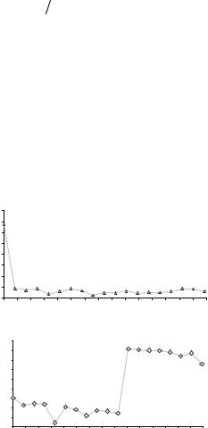
Figure 2.15. AORTIC IMPEDANCE. The calculations made with the data obtained from Figure 2.14 led to these two graphs: impedance modulus above and phase below, both as functions of the frequency expressed in Hertz.
Frequency [Hz]
50 |
Understanding the Human Machine |
the latter being the first component contained in the former.
With 20 beats — of which those shown in Figure 2.14 are part — Figure 2.15 was composed and drawn by means of special software. The upper part plots the moduli while the lower portion is the phase, both as functions of frequency. The whole represents the input aortic impedance. Each point is the average of twenty beats, with a heart rate of 159 beats/min and a peripheral resistance (read it at zero Hz) of 138 mmHg.min/L.
− Two other components
Two other components are present in the hydraulic input impedance: a capacitive-like reactance, XC , and an inductive-like one, XL , both functions of the frequency, the former describing the elastic properties of the vessels and the latter related to the mass of blood in movement. They are also scaled to unit length. Analogous to electric relationships, they are written as,
XC = (1/ ωC) /-90° |
(2.37) |
X L = ωM / 90° |
(2.38) |
and are polar equations which clearly show their moduli, one inversely proportional to the angular frequency, ω = 2πf , and the other directly proportional to it, one with a 90° lead and the other with a 90° lag, as expected in any well-behaved purely capacitive or purely inductive circuit. C is the compliance already introduced before, and M is the mass of blood or inertance, both expressed per unit length of vessel. At lower frequencies, the phase diagram of Figure 2.15 indicates a capacitive dominance, while at higher frequencies the behavior tends to be inductive.
The moduli of the two reactances defined by eqs. (2.37 and 2.38) lead to another parameter, the characteristic impedance of the system, or
ZC = (X L × XC )1/ 2 |
(2.39) |
which is easily read in the impedance modulus plot by averaging out the points beyond the second harmonic.
− Reflections and ventricular-vascular coupling
In an electric line, when there is no reflected wave, the generator internal impedance is equal to the impedance offered by the line (the so called characteristic impedance) and also to the load impedance. It is thus said
Chapter 2. Source: Physiological Systems and Levels |
51 |
that there is impedance matching, with maximum transfer of energy from the generator to the load.
The pulsatile pressure and flow within the arterial tree show significant reflections clearly indicating that, at least from the electrical engineering point of view, no impedance matching is met. It is also obvious that the cardiovascular system is not designed for maximum transfer of energy. In fact, the actual recorded waves — as for example those displayed in Figure 2.14 — are the composition of the forward and of the backward (or reflected) waves (Yin, 1987).
If the heart is the generator and the arterial system is the line connecting it to a load, the question arises as what the optimal or the best coupling between the two is. The subject is still without a definite answer. Authors like O'Rourke, Avolio and Nichols (in Yin's 1987 book) state “Arterial function is optimal when the fluctuation around mean pressure is minimal. Ideal ventricular-vascular coupling entails as low a mean pressure as practicable for adequate organ flow, with as low a mean systolic pressure and as high a mean diastolic pressure as possible. Low mean systolic pressure allows adequate ventricular ejection with low oxygen demands by myocardium and little stimulus to cardiac hypertrophy. High mean diastolic pressure allows adequate coronary perfusion.”
The student is invited to carefully peruse this previous paragraph trying to define and understand each of the concepts mentioned (such as mean arterial pressure, mean systolic pressure and mean diastolic pressure) and the reasons given in each of its sentences. What does cardiac hypertrophy mean? What can stimulate its appearance?
Summarizing: Arterial input impedance is a complex concept graphically presented as modulus and phase, both as functions of frequency. It includes peripheral resistance, elastic vessel properties and the mass of blood. Wave reflection and the coupling between ventricles and their outflow arteries are strongly related to this concept.
To think about and eventually to search in the literature: Where is the major reflection site in the arterial tree? Would an abdominal aortic aneurism or an abdominal coarctation of the aorta affect the hydraulic aortic input impedance? Explain why.
The student is encouraged to review the theory of electric transmission lines in order to find possible analogies with the arterial tree. Recall also that technological hydraulic systems do not show elastic properties in their conduits.

52 |
Understanding the Human Machine |
2.2.1.10. Body fluids
“...all are of the dust, and all turn to the dust again (Ecclesiastes, 3:20) ...
just thirty percent, for the remaining seventy ... it evaporates!”
Blood is indispensable. No wonder that the antiques called it the “elixir of life” and that nowadays encompasses a specialty of its own: hematology. It is part of the body fluids, also and obviously essential for the maintenance of viability, so much that many medical practitioners devote their talents to better handle internal environment derangements (as for example in kidney failure, or severe dehydration). Thus, we will offer here a brief account (McArdle et al., 1991).
Body weight (BW) — a stressing and sometimes pathological concern in the current occidental culture — is composed of two clear-cut parts: solid materials (SM) and total body water (TBW). If referred to body weight, the following simple equation can be written,
100 =[SM / BW +TBW / BW ]100 |
(2.40) |
The first term lies between 30 and 40% while the second one is in the order of 70 to 60%. Hence, most of our body is water. Since 1L of water is equivalent to 1 kg, a person after heavy exercise can easily lose 1, 2 or 3 kg of weight ... which he/she readily recovers when, driven by sheer physiological thirst, he/she drinks the same amount or maybe more. Beware: drink it with some ionic content, otherwise you may run into trouble.
The solid material, in turn, is essentially formed by proteins, P, mostly located in the muscular mass, by minerals, M, mostly held in the bone structure, and by fat, F, distributed all over the body anatomy (and many times showing a prominent concentration in the abdominal volume). Hence, the 30 to 40% of solid material gives way to,
(SM BW )= (P BW )+(M BW )+(F BW ) |
(2.41) |
leaving out the percental 100 for the sake of simplicity. Each term in the right side of the equation above amounts, respectively, to about 18, 7 and 15% in a normal individual. In obese people the amount of fat is larger and that of water smaller.
For those swimming fans: Who floats easier, a lean guy or a rounded fellow? Explain why.

Chapter 2. Source: Physiological Systems and Levels |
53 |
Figure 2.16 summarizes the relationships of the body fluid compartments, including the approximate percentages normally accepted. The upper one states that the extracellular fluid (ECF) and the intracellular fluid (ICF) collect all the body water, or
1 = (ECF TBW )+(ICF TBW ) |
(2.42) |
Both compartments are separated by the cell membrane. The percentages with respect to TBW are, respectively, about 30 and 70%. Hence, all cells are immersed in an internal sea called the internal environment (the famous concept brought up by the French physiologist Claude Bernard in the second half of the XIXth Century). The cells, where all metabolic processes take place, hold most of the fluid. The ECF feeds, cleans and protects the cells. It acts as some sort of buffer. The latter, in turn, is described by the second diagram, where
1 = (IF ECF )+(PV ECF ) |
(2.43) |
The interstitial fluid (IF), i.e., that fluid between cells and outside the capillaries and lymphatic vessels, and the plasma volume (PV) are the components of the ECF. Only a quarter of the extracellular fluid is plasma confined within the cardiovascular system. Plasma volume communicates to the interstitial fluid through the highly permeable capillary
|
TBW |
ECF |
ICF |
30% |
70% |
Cell membrane |
|
PV |
IF |
25% |
75% |
Capillary wall |
Blood cell membrane |
|
|
PV |
CV |
55% |
45% |
|
BV |
Figure 2.16. BODY COMPARTMENTS. TBW = Total Body Water; ECF = Extracellular Fluid; ICF = Intracellular Fluid; PV = Plasma Volume; IF = Interstitial Fluid; CV = Cell Volume in blood. Percentages are referred to TBW, ECF and BV, respectively, from the upper to the lower diagram. Remember that fluid in blood CV is part of ICF. See text for details.

54 |
Understanding the Human Machine |
walls
The volume of plasma is approximately 55% of the total volume of blood, the remaining part are cells (white and mostly red cells). In symbols,
BV = PV +CV |
(2.44) |
or, in relative terms, dividing through by BV and multiplying by 100, |
|
100 =100×(PV BV )+100×(CV BV ) |
(2.45) |
from which two clinically important relationships and concepts come out, the plasmacrit,
Pc =100(PV BV ) |
(2.46) |
and the hematocrit, |
|
Hc =100(CV BV ) |
(2.47) |
both expressed in percent relative to blood volume. For the latter, values below 40% are considered as abnormal. Centrifugation of a blood sample leaves the cell volume packed at the bottom of the tube and plasma on its upper part. It is a simple way of assessing a possible anemic condition.
The Hc includes the fluid contained in the blood cells. If this material is desiccated to remove the water content, then the blood dry weight is obtained.
Exercise: Using the relationships of above, estimate all the presented parameters for a normal male adult of 70 kg. If needed, complement with data taken from any good textbook.
2.2.1.11. Closing remarks
By now, the student should have a fairly good idea of the variables, parameters, organs, and laws involved in the so-called mechanical activity of the cardiovascular system. Some simple exercises were suggested in order to spur curiosity along with a few historical remarks to show how concepts developed with time and knowledge. The text was also interspersed with clinical insights marking, in addition, possible avenues of study and the associated relevant bibliography. A useful practice is to keep a notebook at hand (or in the computer) where those subjects still to be disclosed or clarified are taken down. With time, the student will collect a list that may be helpful when a research project, say, for a doctoral dissertation, has to be decided.

Chapter 2. Source: Physiological Systems and Levels |
55 |
2.2.2. Cardiac Electrical Activity
In this part, the electrical activity of the heart is dealt with, starting with the essential concepts of electrophysiology, continuing with the origin of the heart impulse, its propagation throughout the whole myocardial mass until it is detected from outside by means of surface electrodes to produce the well-known and traditionally used electrocardiogram. Finally, an introduction to changes in the normally rhythmic activity is given. Comments, suggestions and some insights into newer knowledge from molecular biology are also included plus short historical tips. Stimulating the student to put his/her inner drive into action looking back and forward is extremely important.
2.2.2.1. Essentials of electrophysiology
− Model
The electrical phenomena associated with tissue functions, in particular the so-called excitable tissues, fall within the domain of Electrophysiology. Nerves, skeletal, cardiac, and smooth muscles — all excitable tissues — are characterized by a permanent resting and stable electrical state, E1 (Figure 2.17). In fact, such resting condition is so important that, when it disappears, it flags the death of the cell, offering an unmistakable criterion for the experimental researcher to decide whether his/her preparation is still viable (for example, when working with microelectrodes as recording elements). When an adequate stimulus is applied to the cell, the response is a change in the electrical state to another level, E2, re-
|
Adequate |
|
Input |
|
|
|
Output |
|
|||||
|
stimulus |
|
Excitable tissue |
|
|
Response |
|||||||
|
|
|
|
|
|
|
|
||||||
state |
E2 |
|
|
|
|
|
|
|
Output |
|
|||
|
|
|
|
|
|
|
|
||||||
|
|
|
|
|
|
|
|||||||
|
|
|
|
|
|
|
|
|
|
||||
|
|
|
|
|
|
|
|
|
|
|
|
|
|
Electrical |
E1 |
|
|
|
|
|
|
|
|
|
|
|
|
|
|
|
|
|
|
|
|
|
|
|
|
||
|
|
|
|
|
|
|
|
|
|
|
|||
|
A |
|
|
|
|
|
|
|
|
Input |
|
||
|
|
|
|
|
|
|
|
|
|
|
|
|
|
|
|
|
|
|
|
|
|
|
|
|
|
|
|
|
|
|
|
|
|
t0 |
t1 t2 |
t3 |
time |
|
|||
Figure 2.17. MODEL OF AN EXCITABLE TISSUE. The output has an electric stable resting state, E1, and a metastable state, E2, after an adequate stimulus is applied as input. The time the second state is
kept, td = (t3 – t2), depends on the character-
istics of the tissue. Thus, the behavior reminds of an electronic monostable flip-flop.
56 |
Understanding the Human Machine |
maining at it for a very specific length of time, td = (t3 – t2), which exclusively depends on the characteristics of the tissue. It reminds the behavior of an electronic monostable multivibrator (mono = one). The time difference between t2 and t0 is called the latency, that is, it measures how long it takes the cell to react to the stimulus and is also a characteristic of the tissue. The amplitude of the cell response, the action potential, is obviously the difference of the two electrical levels, E2 and E1.
In the laboratory environment, the stimulus is produced and controlled by an external equipment (biological stimulator) and usually it is of rectangular shape, defined by an amplitude, A, either in volts or amps, and width (t1 – t0), in ms, both adjustable at will. In the physiological normal situation, action potentials act as stimuli, although their actual shape may deviate considerably from the ideal rectangular waveform.
Small research subject: Stimuli other than the electric type can elicit a response in excitable tissues. Find out which. Mention three more. Hint: Think in terms of types of energy. Did you accidentally hit your elbow experimenting a nasty electric sensation? Explain.
− Resting membrane potential
Most of the cells of excitable tissues are long and cylindrical in shape surrounded by a membrane, about 100 Å thick (1 Å = 10–8 cm), which separates the intracellular fluid (ICF) and its contents from the extracellular fluid (ECF). When a very small diameter electrode (a microelectrode, of about 1µm) — connected to one of the inputs of a special high impedance amplifier — is introduced into the ICF puncturing the thin cell membrane while the other amplifier terminal is hooked to a return electrode immersed in the ECF, the recording instrument (a dc coupled oscilloscope) shows a displacement of the base line from the zero level to about –80 to –90 mV, assuming that the excitable cell (say, a skeletal muscle one) is alive. This is the resting membrane potential
or the stable electric state, E1, already introduced above. The internal side of the membrane is negative with respect to its external counterpart.
This |
highly summarized |
description is |
an |
experimental fact |
that |
can |
be demonstrated in |
any laboratory |
of |
electrophysiology. |
The |
ECF contains a high concentration of sodium ions and a low level of potassium ions. Conversely, the ICF shows a low level of sodium and a high concentration of potassium. Both ions on both sides of the membrane are also accompanied by chloride ions. The membrane is relatively permeable to all these charge carriers; however, it does not permit the passage of large proteic anions, which abound within the cell. Besides,
Chapter 2. Source: Physiological Systems and Levels |
57 |
the membrane is a good insulator constituted by oriented proteins and phospholipids, roughly containing one ion per 5,000 water molecules. ECF and ICF, instead, have in the order of one ion per 175 water molecules, meaning that these fluids are by far better electrical conductors.
Study subject: The student should check in any physiology textbook the values reported for sodium, potassium, chloride and proteic ions in ECF and ICF, in nerve and skeletal muscle cells. Via INTERNET, we suggest DEVELOPMENT OF TRANSMENBRANE RESTING POTENTIAL, by David L. Atkins, Professor of Biology at George Washington University, atkins@qwis2.circ.qwu.edu, 1998. Calculate also the electric field, in volts/meter, stressing the cell membrane. Compare it with porcelain. Review also the fluid compartments. Notice that the ECF faced by the excitable cell membrane is its interstitial fluid part IF, with no proteins. Plasma, instead, the other portion of ECF, contains a large amount of proteins and is exclusively restricted to the cardiovascular system.
− Resting potential by the Ionic Theory
On December 20, 1998, Sir Alan L. Hodgkin died in his home residence of Cambridge, England, at the age of 84. He was 1963 Nobelist in Physiology or Medicine for his analysis of the ionic basis of the action potential, former Master of Trinity College in Cambridge University and President of the Royal Society. Co-recipients of the prize were also Andrew Fielding Huxley and John Carew Eccles, the latter from Camberra, Australia. However, many others have also contributed to the ionic theory and a few of their names will be mentioned here (such as Kenneth S. Cole and Bernard Katz). Some classical and enlightening references for the interested student are Hodgkin (1964), Katz (1966), Cole (1982) and Gardner (1992). Even though there are still a few who question the validity of the theory, most of the scientific community has accepted it and continues to work in its improvement.
Figure 2.18 represents the cell membrane with two vertical lines. On the left, there is the ICF, i.e., inside the cell, and on the right we have the ECF, which coincides here with the interstitial fluid. The former is essentially a compartment high in positive potassium and negative proteic ions while the latter is characterized mainly by a high concentration of positive sodium ions. Potassium and sodium cannot exist as such just by themselves because they appear from electrolytic dissociation of chemical compounds, in this case, of KCl and NaCl. Hence, both compartments also have their chloride ionic counterparts as the proteic anions in the ICF have theirs, in such a way that, on both sides, the neutrality principle must be met, that is to say,
Sum of all positive charges = sum of all negative charges or