Understanding the Human Machine - A Primer for Bioengineering - Max E. Valentinuzzi

during ooycte development from the preantral stage oocyte to the metaphase II stage.

Electrical measurements were recorded as the potential difference between a 3 M KCl Ag/AgCl microelectrode (tip impedance of 20 MΩ) inserted into the oocyte and an external 3 M KCl glass electrode located downstream of the oocyte. Electrodes were coupled to a dual channel high input impedance amplifier. Recordings were displayed on a digital storage oscilloscope and stored to the hard drive of a PC.

The paper of Emery, Miller and Carrell (2001) has been the main source of most of this material. The interested student can find more details about the subject in the papers by Okamoto, Takahashi and Yamashita (1977), McCullough and Levitan (1987), and Mattioli, Barboni, Bacci et al. (1990).

3.2.2. Traditional Bioelectrical Signals

In electrophysiological studies, concerned with the traditional excitable tissues mentioned above, action potentials are commonly recorded by means of microelectrodes (in research laboratories) or small electrodes (in research or clinical laboratories). The duration of these signals vary enormously from one tissue to the other; say, from 0.1 ms in nerve and skeletal muscle up to 300 or 400 ms in cardiac muscle. In smooth muscle, the duration can reach 500 ms with rather unstable resting potential. Smooth muscle is responsible for the contractility of hollow organs, such as blood vessels, the gastrointestinal tract, the bladder, or the uterus. Its structure differs greatly from that of skeletal muscle, although it can develop isometric force per cross-sectional area that is equal to that of skeletal muscle. However, the speed of smooth muscle contraction is only a small fraction of that of skeletal muscle.

The traditional electrical signals recorded with relatively large electrodes are the electrocardiogram (ECG), the electromyogram (EMG) and the electroencephalogram (EEG).

The ECG was described and discussed with enough detail in Chapter 2, Section 2, Part 2 and, thus, there is no need to elaborate further in the subject. Its origin is located in the heart cells. It has been fully established during the course of the XXth Century and is widely and routinely used all over the world as important, easy and inexpensive diagnostic tool.

Let us now go into the electromyogram (EMG) and the electroencephalogram (EEG), as the other two bioelectric events that have won wide clinical acceptance.

3.2.2.1. The EMG

When a muscle contracts, small electric potentials are produced. If normally innervated, the muscle shows no electrical activity at rest. Surface or needle electrodes can sense such potentials, which are usually proportional to the level of the muscle activity. The signal detected by the electrodes is amplified and recorded and is known as the electromyogram. The EMG signal is virtually meaningless “as is;” however, when properly analyzed, considerable information can be retrieved from it (Figure

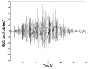
Figure 3.5. ELECTROMYOGRAM. Typical EMG recorded from a 40 yrs old female. The subject stood up to perform lateral abduction-adduction of one arm. Initially, both arms rested hanging down. Hence, the record displays the sequence of lifting and lowering the arm from 0° to 90° and back to 0°. The amplitude of the signal increases with abduction and decreases with adduction. For the same angle, such amplitudes were smaller when the arm was returning to its resting position than when it was being lifted. An angular scale was drawn behind the subject in 10° steps, from 0 (hanging arm) to 90° (the latter corresponding to a horizontal extended arm). A pair of sterile stainless steel acupuncture needles was used as electrodes (0.2 mm in diameter), inserted in the belly of the deltoid medium with a separation of 2 cm. Abduction corresponds to the first left half and adduction to the second portion. Sampling frequency was 3 kHz. The vertical axis is calibrated in rms mV while the horizontal axis corresponds to time. Record obtained at the Department of Bioengineering, UNT, 1997.

3.5).

The EMG is a rather ubiquitous tool used, for example, as a measure of muscular effort in traumatology, as an evaluation parameter in rehabilitation engineering, as the control input to myoelectric prostheses and as another diagnostic piece of information in nerve damage or injury caused by a compressed disk in the neck or back, nerve compression from carpal tunnel syndrome, myopathies many times faced in clinical medicine, neuromuscular diseases, inflammation or degeneration of peripheral nerves caused by conditions such as diabetes, pernicious anemia, and heavy metal toxicity. It can also be used to estimate the muscle action potential propagation velocity (Geddes and Baker, 1989; Spinelli, Felice, Mayosky et al., 2001).

The presence, size, and shape of the waveform produced on the oscilloscope (often combined with sound output via a loudspeaker) provide information about the ability of the muscle to respond to nervous stimulation. Each muscle fiber that contracts produces an action potential and the EMG is the compounded signal of many individual action potentials. This electrical activity of skeletal muscle can be described mathematically as a random process, which is amplitude modulated. When muscular effort is low, the amplitude of EMG is low; when muscular effort is high, the amplitude of EMG is high. Thus, better estimates of EMG amplitude improve the ability to determine the activation level of muscles. Active research in applied signal processing and stochastic estimation is being used to improve methods for estimating the amplitude of EMG signals (Clancy, 1999; Clancy & Hogan, 1994; 1995; 1997; Clancy and Farry, 2000; Clancy, Morin and Merletti 2002).

Since EMG is essentially a by-product of muscle contraction, it is logical to try to relate the electrical activity of muscle to its mechanical activity. Joint torque is frequently selected as the mechanical activity, as it is easy and reliable to measure. By and large, as the number of active motor units is increased and/or the average firing rate of active motor units is increased, both EMG amplitude and total muscle tension increase. However, the relationship is dynamic and may also need to be treated as nonlinear.

When a muscle fiber loses its nerve supply, it exhibits a characteristic irritability manifested as spontaneous discharges at rest. Single muscle

discharge, called fibrillations (not related at all with cardiac fibrillation) have a short duration (.5 to 1.5 msec), low amplitude (50–300 microvolts) and a rather regular rhythm. After denervation, it takes some time for fibrillation to appear; this appearance time is species-dependent (about 3 days in mouse, 4 in the rat, 6 in the rabbit, 8 in the monkey and up to 18 days in humans). Thus, the higher the rank in the zoological scale, the longer the time. If reinnervation does not occur, the muscle fibers atrophy and the fibrillation potentials disappear. If reinnervation takes place, the fibers cease to atrophy and the fibrillation potential gradually disappear, being replaced slowly by normal muscle action potentials which show up when a voluntary effort is made or when the muscle is contracted reflexively (Geddes & Baker, 1989).

Muscular fibrillation is abnormal but is not characteristic of any single disease. They may be seen whenever a muscle cell membrane becomes hyperirritable. If they are widespread in all four extremities and consistent with the clinical history, amyotrophic lateral sclerosis (or Lou Gherig's disease) should be suspected. However, there is a great deal of subjectivity in the interpretation of an EMG. Polyphasicity (that is, more than 5 baseline crossings on an EMG) and increased serration may be seen in reinnervated muscles or primary myopathy; in most of them (such as myotonic dystrophy), however, amplitude is reduced and the action potential prolonged.

The student is advised to review the background material in electrophysiology, the concept of motor unit and the basics of skeletal muscle physiology. Something can be found in the preceding chapter, in Geddes and Baker (1989), in any physiology text, or in the WEB.

3.2.2.2. The EEG

Geddes and Baker (1989) produced a clear account of this subject. Some of the material that follows has been taken from these authors. See also Nuñez (1981) and Sharbrough, Chatrian, Lesser et al. (1991) As usual, the WEB is another place where more information can be readily found.

The electrical activity of the brain is recorded with three types of electrodes: scalp, cortical and depth. With scalp electrodes, the recording is called an electroencephalogram (EEG). If the electrodes instead are placed on the surface of the brain, the recording is an electrocortigram (ECoG). If electrodes are advanced into the brain, the term depth re-

cording (DREEG) may be used. With the latter, and surprisingly, little damage if any is caused. Any of these signals recognizes its origin in the activity of numerous neurons with fluctuating membrane and action potentials. All three techniques are examples of extracellular recording.

R. Caton, in 1875 and 1887, was apparently the first one to report spontaneous electrical activity from the brain of a variety of animals (Geddes and Baker, 1989); however, he only provided good verbal description of the phenomenon. It was Berger, in 1929, who obtained graphic records using Einthoven’s string galvanometer and scalp electrodes. His papers went largely unnoticed until Adrian and Matthews, in 1934, in Great Britain, and Jasper and Carmichael, in 1935, in the USA, reviewed and confirmed his earlier findings. A complete account of the development of electroencephalography was published under the editorship of Rémond (1971).

As figures 3.6 and 3.7 illustrate, the electroencephalographic signal looks like noise, although a normal EEG shows a dominant frequency of about 10 Hz and amplitude in the range of 20 to 200 µV. This activity, which is called the alpha rhythm, ranges in frequency from about 8 to 13 Hz and is most prominent in the occipital and parietal areas. The alpha rhythm increases in frequency with age from birth and attains its adult appearance by 15–20 years of age. It is most salient with the eyes closed and in

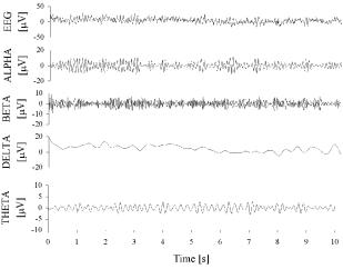
Figure 3.6. ELECTROENCEPHALOGRAM. EEG´s showing a regular normal signal and typical alpha, beta, theta, and delta rhythms. Records obtained at the Department of Bioengineering, UNT, 2003.

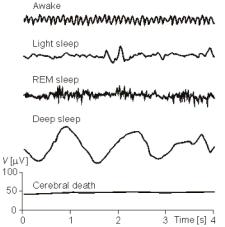
Figure 3.7. EEGs DURING DIFFERENT CEREBRAL CONDITIONS. The subject is awake (upper channel), lightly asleep (second channel), asleep under conditions of rapid eye movement or REM (third channel), and in deep sleep (fourth channel). A flat EEG means cerebral death and represents the criterion followed to decide donation of an organ. Downloaded from the WEB, freely available.

the absence of concentration. Opening the eyes or performing a cerebral activity, such as mental arithmetic, decreases or abolishes the alpha rhythm. There are other waveforms such as the beta, delta, theta and spikes (Figure 3.6). Their interpretations belong to the specialist and lie beyond the introductory scope of this text. Sleep has also important reflection on the EEG (Figure 3.7), so much that there are laboratories that specialize in it, particularly to study its many disturbances.

From a physical point of view, the EEG can be modeled as a finite sum of harmonic oscillations at discrete rates triggered by a central pacemaker. Hence, brain waves can be interpreted as consisting of a fundamental oscillation superimposed to higher harmonics. In terms of this concept, brain waves are composed of a series of simple sinusoidal waves ranging in frequency between 0.25Hz and 64Hz (7 octaves; doubling a given frequency defines an octave, say, from 250 Hz to 500 Hz, and it is a term widely used in music), whereby the full composition essentially depends on the state of consciousness, such as wakefulness or sleep stages. Thus, the EEG can help diagnose seizure disorders like epilepsy, head injuries, brain tumors, encephalitis, some kinds of infections, metabolic disturbances, and sleep disorders.

The number of nerve cells in the brain has been estimated to be on the order of 1011. Cortical neurons are strongly interconnected. Here, the surface of a single neuron may be covered with 1,000–100,000 synapses. The electric behavior of the neuron corresponds to the description of ex-

citable cells introduced earlier in the book. The current density associated with neuronal activation produces an electric field, which can be measured, as mentioned before, on the surface of the head or directly on the brain tissue. For most excitable tissue the basis for the current density is the propagating action potential, for the EEG, instead, it appears to arise from the action of chemical transmitters on postsynaptic cortical neurons. The action causes localized depolarization or hyperpolarization with the net result in either case of a spatially continuous volume source distribution, because neural tissue is generally composed of a very large number of small, densely packed cells. Theoretical models have been developed using electric field theory.

There is an international standard system to record the spontaneous EEG. In it, 21 electrodes are located on the surface of the scalp. The positions are determined using as reference points the nasion (delve at the top of the nose), and the inion (bony lump at the base of the skull on the midline at the back of the head). From these points, the skull perimeters are determined and they are divided into given intervals. Besides the international system, many other lead systems exist for recording electric potentials on the scalp. Bipolar or unipolar electrodes can be used in the EEG measurement. In the first method the potential difference between a pair of electrodes is measured. In the latter method the potential of each electrode is compared either to a neutral electrode or to the average of all electrodes. Guidelines for EEG-recording are periodically revised and published by the American Electroencephalographic Society (see, for example, Journal of Clinical Neurophysiology, 1994, January issue).

3.2.3. Biomagnetic Signals

Magnetobiology and Biomagnetism, the former dealing with the effects of external magnetic fields on biological systems while the latter studies only magnetic fields generated by these systems, has taken a clear objective and well-defined path in the last 40 or 50 years, after being mixed unfortunately for a very long time with pseudoscience and charlatanism (Valentinuzzi, 2002). There are several research groups in the USA, Finland, Japan and Brazil seriously working in this fascinating area applying top technologies.

Biomagnetic sources can be found in electric currents (as action potentials generated by excitable tissues), in diamagnetic and paramagnetic

substances in the body, and also in the presence of ferromagnetic substances found or injected as tracers in the organism. We should mention also the well-documented existence of magnetic bacteria, found sometimes in sewage waters. These signals are akin to electrical signals so that, collectively, we might speak of bioelectromagnetic signals.

The following smaller case paragraphs very succinctly describe the three types of substances found in nature and in living organisms according to their magnetic properties.

Diamagnetic substances are expelled from a magnetic field, i.e., they are displaced from the points of greater intensity to those of lesser intensity. If the body they form is elongated in shape, then it is positioned (while suspended) with its longest axis oriented transversely to the direction of the field. The field inside these substances is weakened. Antoine Cesar Becquerel (1788–1878) —founder of a dynasty of distinguished scientists— worked and corresponded with Faraday on diamagnetism. He had noticed examples of it (around 1827) before Faraday (who did it circa 1847) but had failed to generalize from them. Michael Faraday (1791–1867), instead, had a clearer understanding of the phenomenon. In fact, he coined the words “dia” and “paramagnetic”. Alexandre Edmond Becquerel (1820–1891) was the second son of Antoine Cesar. From 1845 to 1855, Edmond devoted most of his attention to the investigation of diamagnetism.

Paramagnetic substances are sucked in by a magnetic field, i.e., they are displaced from the points of lesser to the points of greater intensity, and a body of such material is lined up with its greater axis in the direction of the field, reinforced in its interior (field lines are more concentrated). The study of paramagnetism is mainly due to Pierre Curie (1859–1906). In fact, he studied the three groups of substances: ferromagnetic, such as iron, that always magnetize to a high degree; low magnetic, or paramagnetic substances, such as oxygen, palladium, platinum, manganese, and several salts, which magnetize in the same direction as iron but much more weakly; and also diamagnetic substances, which include the largest number of elements and compounds (many are biomaterials). Curie concluded that diamagnetism must be a specific property of atoms. It exists also in ferromagnetic or paramagnetic substances but is little apparent there because of its weakness. Ferromagnetism and paramagnetism, on the other hand, are properties of aggregates of atoms and are closely related. The ferromagnetism of a given substance decreases when the temperature rises and gives way to a weak paramagnetism at a temperature characteristic of the substance and known as its “Curie point”. Paramagnetism is inversely proportional to the absolute temperature. This is Curie’s law. A little later, Paul Langevin, who had been Curie’s student at l’ École de Physique et Chimie, proposed a satisfactory theory by postulating a thermal excitation of the atoms in the phenomena of magnetization. These are concepts that still constitute the basis of modern theories of magnetism.

Ferromagnetic substances intensify the field extraordinarily. The reinforcement can be thousands of times greater than in the case of paramagnetic substances. The bodies made of

of these substances deform the lines of force to such an extent that the former tend to get nearer to the poles of the magnet generating the field.

When a paramagnetic body is placed in a magnetic field, it also acquires diamagnetism, so that there is a superposition of both properties. To elucidate accurately the value of paramagnetism, it is necessary to make corrections relative to diamagnetism. Paramagnetism always conceals diamagnetism by virtue of its greater intensity. Ferromagnetic bodies are less common in nature than the paramagnetic bodies. Ferromagnetism can be considered a special form of paramagnetism, which manifests when matter acquires a cristalline structure and depends on the intensity of the magnetic field.

The three variants of magnetism (dia-, paraand ferro-) may be characterized by the concept of magnetic permeability, which becomes larger when going from diamagnetism to paramagnetism to ferromagnetism.

Magnetic permeability is related to the concept of magnetic susceptibility. There is a well-known mathematical formulation that the student probably already saw in physics courses. This magnetic characterization of substances or materials in general becomes relevant to their respective behaviors when an external magnetic field is applied to them. Physiological or injected magnetic tracers can be detected with susceptometric measurements, as for example iron in liver (Carneiro, Baffa et al., 2002). Such signals may help in the study of stomach motility (Carneiro, Baffa & Oliveira, 1999) or in the generation of images of the gastrointestinal tract (Moreira, Murta and Baffa, 2000).

Akin to the electrocardiogram, the electromyogram and the electroencephalogram, we can easily envision the existence of a magnetocardiogram (MCG), a magnetomyogram (MMG) and a magnetoencephalogram

(MEG), since the three former, respectively, are time changing electric phenomena. In other words, ion currents in excitable tissues sustain very weak magnetic fields, and this phenomenon stands above the shoulders of Hans Oersted, who back in 1820, demonstrated that an electric charge in motion through a conductor (i.e., a current) sets up a magnetic field. This is basic physics knowledge.

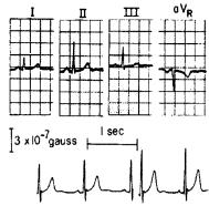
Baule and McFee, in 1963, recorded the fluctuating magnetic field produced by the heart so taking the first magnetocardiogram (MCG). They found it had a maximum of about 5×10–7gauss at the peak of the QRS complex. The earth’s steady magnetic field strength is in the order of 0.5 gauss; by comparison, the heart maximum magnetic field, at several centimeters from the torso, is only about one millionth of the earth’s field. Magnetic disturbances or noise in an urban environment can easily be greater than 10–4 gauss. Thus, sophisticated technology is mandatory to extract the weak MCG from this much larger background interference. Since its inception, important advances have been made in biomagnetic instrumentation. The most important is the development of shielded rooms and ultrasensitive magnetometers based on the superconducting quantum interference device (SQUID). Description and discussion of the necessary technologies are by far beyond the objectives of this textbook and the reader, if interested, should search the specialized literature. The literature is extensive and several reviews are available, as for example, Williamson, Hoke, Stroink et al. (1989). Despite the similar appearance of MCG and ECG waveforms, MCG typically shows greater spatial variation and can potentially provide improved localization of sources (Cohen and Chandler, 1969). In addition, MCG is sensitive primarily to tangential sources while the ECG is more sensitive to radial sources. Thus, additional information may be expected (Verzola, Baffa, Wakai et al., 1995). Figure 3.8 illustrates a MCG picked up with a coil perpendicular to the chest of a subject.

Figure 3.8. MAGNETOCARDIOGRAM. This MCG was taken with the coil axis normal to the chest in two different positions relative to the heart; the ordinate is proportional to the induced magnetic field. The upper channel shows the simultaneously recorded ECG. Courtesy of Dr. David Cohen, MIT, Boston.