Understanding the Human Machine - A Primer for Bioengineering - Max E. Valentinuzzi

but inspection of Figure 2.5 easily shows that sin α = H/R which, after substitution in eq. (2.6), ends up in

which describes in the plane the statement in italics given above. Now we face an arguable step:

For one principal plane containing the principal radius R1, we have T1 = P×R1 , which is eq. (2.7); for the other, perpendicular to the former, and following exactly the same rationale as developed above, we obtain, T2 = P×R2. Solving each for P and adding them up leads to,

because pressure, by Pascal’s Law of hydrostatics, has to be the same. Moreover, if it is accepted that T1 = T2 = Tp and defining T = Tp/2, we end up with

The latter equation is fully coincident with eq. (2.2). The weakness in the last part of the derivation is pointed out and, therefore, left to a more inquisitive (and powerful) young mind as a possible “little project”. Tensors might supply a good tool for it.

If the balloon is a sphere, the two radii are equal to R and eq. (2.9) reduces to the well known T = PR/2. If now the concept of wall stress is introduced in a balloon or hollow organ with wall thickness, h, as defined above in (2.3), we get,

always keeping in mind the existence of a proportionality constant. Its numerical value should be determined for each particular case without worrying about the come and go of a 2 in it. In the heart, intraventricular hypertension and ventricular dilatation increase wall stress (a risky condition); with time, such hypertension produces hypertrophy, meaning a thickening (larger h) of the ventricular wall, obviously tending to relief parietal tension. Hence, hypertrophy is a compensatory mechanism.

Suggested exercise: Search in the published literature a possible value for left ventricular volume in an adult healthy man. Thereafter, calculate the equivalent diameter (as if it were a sphere).

Suggested exercise: Applying Laplace’s Law, estimate the ratio of left ventricular wall thickness, hL, to right ventricular wall thickness, hR. Explain the result.

2.2.1.6. Vessels: arteries and veins

By definition, artery is a vessel carrying blood from the heart to the periphery and vein is a vessel carrying it back to the heart, irrespective of whether it is or not well oxygenated. Figure 2.2 displays the arterial section on the right and the venous section on the left. Well embedded in the different tissues is the microcirculation, which includes (i) the last and smallest in diameter (the arterioles) portion of the arterial side; (ii) the capillaries, as the only exchange section through their highly permeable thin walls; and (iii) the first and smallest in diameter (the venules) segment of the venous side. The microcirculation constitutes a separate chapter of utmost importance in vascular physiology. One of the most remarkable properties, especially in beds like the brain, heart or kidneys, is the ability to control the amount of blood reaching the network. This is called autoregulation, independent of mechanisms controlled by higher centers.

Unlike any technological hydraulic system, all blood vessels are elastic, a property bestowing upon them a powerful regulatory tool, both as passive mechanism and also as an active one via smooth muscles covering the external side of their walls. One way to evaluate passive elasticity is by application of the concept of compliance, C, defined as,

that is, the differential change in volume V per differential change in pressure P. Its units, as expected, are for example [cm3/mmHg]. The inverse of C is called elastance, E. One of the several reported values for the latter in normal men puts it in about 1,500 dynes/cm5. The interested student will find more details in the current literature, as for example, other definitions to describe the elastic properties that, interestingly enough, have been kept essentially the same over the years (Valentinuzzi, Ghista & Nichols, 1979). Mostly, newer reports refer to the action of drugs on these parameters or to the relative contributions of elastin and collagen components (Armentano, Cabrera Fischer, Levenson et al., 1990; Armentano, Levenson, Barra et al., 1991; Cabrera Fischer, Levenson, Barra et al., 1993).

A vessel with high compliance increases greatly its volume with a small increment in pressure. Veins are much more compliant than arteries and, as a consequence, most of the blood volume (about 8% of body weight) lodges dynamically within the venous system.

Suggested exercise: A person is placed horizontal in a centrifuge with his legs pointing to the center and his head pointing outwardly. After rotation during a while, is he still alive? If not, could you explain why? (It sounds weird and awful, but it is descriptive).

Study subject: A reference is given above (Armentano, Cabrera Fischer, Levenson et al., 1990). In its title, it mentions “the aortic elastic response to epinephrine”. What is such response? Think in terms of an athlete who is getting ready to act.

Do you remember Hooke's Law of elasticity? Try to correlate it with eq. (2.11) above.

Another characteristic of the circulatory vessels is their smooth musculature. These muscles are controlled by the autonomic nervous system and by hormonal secretions of different kind and origin. These muscles modify the vessels’ caliber or lumen (see the suggested study subject above). Hence, the compliance of a vessel in active state is different than its compliance when inactive. Moreover, in some vascular disease conditions (such as arterosclerosis, flebitis, varicose veins) compliance of the vessels is significantly modified. In arterosclerosis, compliance decreases (arterial hardening) while in varicose veins, vessels tend to be overcompliant.

Study subject: Compare the musculature of arteries and veins. What part of the vascular system is the most heavily covered with smooth muscle? Where is peripheral resistance mostly concentrated on?

2.2.1.7. Cardiac output or the total flow, coronary and cerebral flows

− The direct Fick method

In a previous section above, blood flow was presented as one of the variables in the CVS. Here, we want to be more specific. The total flow or cardiac output — CO = Ft — exits the left ventricle at high pressure, enters the right heart via the vena cava at very low pressure, is also expelled by the right ventricle at moderately low pressure, and finally returns to the right atrium at very low pressure again (Figure 2.2 and Figure 2.3). If the lungs are considered as a node (Figure 2.6), the Continuity Principle applied to blood (as carrier, in mLblood/min) and oxygen (as transported substance, in mLO2/mLblood) establishes in the steady state condition that,

where [V] and [A], respectively, stand for the concentration of oxygen in venous and in arterial blood, while Fox represents the net oxygen uptake in [mLO2/min] via the respiratory system. Solving for Ft, results in,

Oxygen Input + [mL/min]

Figure 2.6. FICK’s PRINCIPLE. In the steady state, everything that goes in (per unit time) must also go out. See eq. (2.12) and text.

which is the famous and well-known Fick’s formula (Hoff and Scott, 1948). Those familiar with electric circuits will find this similar to the total current converging to and diverging from a node. After all, recall that current is nothing but amount of electric charge per unit time (1 amp = 1 coulomb/s) and in eq. (2.12) we have amount of oxygen also per unit time. The numerator in eq. (2.13) is usually obtained from a metabolimeter (an easy measurement). A normal adult at rest may take about 250 mLO2/min. A sample of blood from any artery (the method, thus, requires arterial puncture) and, subsequent determination in the biochemistry lab, gives the arterial concentration of oxygen. The venous concentration of oxygen is not easy. Samples from a peripheral vein are not acceptable because the oxygen consumption varies from tissue to tissue. A representative sample has to be a mixture coming from all tissues. Only the right atrium, or better, the right ventricle, or the best, the pulmonary artery, carry venous blood meeting such requirement. Hence, a probing catheter must be introduced to any of these vascular places in order to withdraw a few milliliters of blood to be tested in the lab for oxygen content. Typical expected normal values are 20 mLO2/100 mLblood, for the oxygenated blood, and about 15 mLO2/100 mLblood, for the mixture of venous blood. Thus, the arteriovenous difference is about 5. These units are many times referred to by physiologists as 15 volume percent. When the above figures are replaced in eq. (2.13), the result is a steady state value of 5 L/min.

Adolph Fick described the method in 1870 in a very short communication to the Society of Physics and Medicine of the city of Würzburg, in Germany (Hoff and Scott, 1948, see pp 26–31). However, he never actually put it into practice because he lacked the means to do it. Human cardiac catheterization was still many years ahead, even though Claude Bernard, on one hand, and Jean Baptiste Auguste Chauveau and Etienne Jules Marey, on the other, all three in France, performed it almost routinely in animals. Fick's idea was first tested in dogs by H. Gréhant and C.E. Quinquaud, in 1886, who reported values of 591 to 2,614 mL/min for body weights ranging from 7 to 18 kg. Zuntz and Hageman, in 1898, did it in the horse. It was Werner Theodor Otto Forssmann, in 1929, the first to introduce a catheter in his own right heart via the brachial vein, so demonstrating the feasibility of the procedure in the human being. He got later on, in 1956, shared with A. Cournand and D.W. Richards, the Nobel Prize, although at the moment he was severely reprimanded by his superior medical chief for breaking hospital rules. Finally Klein, in 1930, measured cardiac output in man by the direct Fick method (this is the way it is now called) obtaining venous samples with a cardiac catheter. It took 60 years (1870–1930) to reach the human application. Insufficient technology was obviously a factor against, but not enough basic knowledge was undoubtedly another (the human heart was perhaps viewed as some kind of “untouchable”). A third one may have been the relatively slowness of communications (as compared to those we enjoy nowadays). A nice epistemological little research project.

− The indicator dilution method

Even though it is a reference considered for many years a Gold Standard, the direct Fick method is not practical. Using an exogenous indicator (such as dye, radioactive substance, saline or heat), suddenly injected at a given site in the circulatory stream (peripheral vein, right ventricle or left ventricle), a dilution curve can be detected in a peripheral artery. Such curve, continuously recorded, contains information from which cardiac output can be obtained (Geddes and Baker, 1989). A basic condition is that the indicator bolus must traverse at least once the central pump or duct, either the left or the right.

Figure 2.7 represents a hydraulic and simplified model (which can actually be built and tested). It is composed of a pump, a main duct carrying the total flow Ft, a number of branches (1, 2, ..., j, ... n), and a return pipe back to the pump with the same flow. Thus, it is a closed leakless circuit. By injecting a known weight mi of indicator in one branch and by detecting the passage of the indicator in another branch, after passage through the pump, the total flow can be determined. The calibrated detector, with its associated recording equipment, provides the dilution curve from which the necessary data are extracted.

Under ideal conditions, the indicator will be uniformly mixed after injection in a small liquid cylinder of length xk and cross sectional area Ak.

Figure 2.7. HYDRAULIC AND SIMPLIFIED MODEL. It is composed of a propelling pump, a main outflow, n branches and a return line. I and D are, respectively, the injection and detection sites. An adequate transducer and recording system produce an ideal concentration versus time output.

The cylinder will move along the branch and appear in the main return conduit at, say, point J, where the amount of indicator will be now uniformly dissolved in a new cylinder of length x and cross-sectional area A. This cylinder of volume V = xA will advance at a velocity x/t , where t is the time required for the cylinder to progress a distance equal to its own length. Multiplying the latter by A, leads to Ft = Ax/t = V/t. On the other hand, the concentration of indicator within the cylinder is C = mi/V which, combined with the former and solved for flow, results in,

so offering a first expression relating total flow with indicator mass, concentration and time, the two latter derived from a highly inconvenient place in the circulation. Our little ideal cylinder proceeds its travel, gets through the pump, reappears at the main outflow and, after reaching the multiple branching off site at point K, it breaks off too into as many new cylinders as branches in the circuit. Each branch cylinder will take a portion mj of the injected mass in such a way that the total amount emerging at point J should satisfy the Conservation of Mass Principle, that is,

where j stands for any branch of the system of n branches. Besides, the total flow will be equal to the sum of all branch flows (once more the Continuity Principle). If the detector is located in branch j = n, at a time ta (appearance time), it will begin to detect the passage of a cylinder of length xj and cross-sectional area Aj , which moves at velocity xj / tj , car-

rying an amount mi of indicator dissolved in its volume Vj . The time tj is the time required for the cylinder to move a distance equal to its length. If the velocity equation is multiplied by the cross-sectional area of the branch, the flow in branch j is obtained, i.e.,

where Vj = Aj xj is the volume of the j-th cylinder carrying a concentration Cj = mj / Vj. It must be emphasized that the latter branch concentration is what the recording system supplies. Since uniform distribution was assumed and since sharp borders of the cylinder are supposed, the ideal dilution curve will be a perfect rectangle, ranging from a minimum to a maximum, the difference Cj being the concentration in the cylinder (Figure 2.7). The time difference, tf – ta , is known as the passage time tj .Combining eq. (2.16) with the above branch concentration leads to the branch flow, or

neither equal nor to be confused with the total flow Ft but obviously similar to eq. (2.14).

If now eqs. (2.14) and (2.17) are considered, recalling also the total flow as the sum of the partial branch flows, we can easily write,

Each side of eq. (2.19) is a polynomial in mj and, by using a corollary of a theorem of algebra, it can be seen that this equation is true only if the corresponding coefficients of mj are equal, so that,

meaning that in eq. (2.14) the denominator can be replaced by Cj tj and, thus, resulting in

The latter equation is called the Stewart–Hamilton formula, widely used in the determination of the average cardiac output. It is based on the property described by the previous eq. (2.20): the area under the dilution curve recorded at any peripheral artery is always equal to the area recorded under the main outflow (Valentinuzzi, Geddes & Baker, 1968).

In actual situations, the indicator bolus is obviously not a cylinder. It has a drop-like shape, with a head and a long tail, tending to become longer as it advances within the conduit. Someone likened it to a huge spermatozoid. The concentration shows a maximum slightly behind the front edge decreasing steadily as one explores further back in it. This describes concentration as a function of the longitudinal axis of the bolus. Consequently, a detector, fixed in a given place, will see the bolus as it passes under producing an experimental concentration versus time dilution curve with a clear rise time, a maximum and a long tail (Figure 2.8). The area under the curve is expressed mathematically as the integral of the concentration curve as a function of time, from the beginning of the curve (appearance time) up to the end (final time). The latter should be at infinity, but for practical reasons is usually defined as the time when the concentration drops to 1% of the maximum level (tf = t1%). By dividing the area (graphically obtained) into the time difference or base of the dilution curve, an average concentration results and, thus, an equivalent ideal rectangle is produced (Figure 2.8). In such a way, we can have a

Drop-like shape of the bolus

Figure 2.8. ACTUAL SHAPE OF THE DILUTION CURVE SHOWN AS A FUNCTION OF TIME. Usually, the end of the curve is taken at the 1% level with respect to its maximum value.

good graphic correlate of eq. (2.21). More properly, however, it is to rewrite the latter as,

where c(t) stands for the concentration function whose explicit mathematical form is not known, except for empiric approximations (Valentinuzzi, Valentinuzzi & Posey, 1972), and is only obtained graphically after performing an experiment. The difference, tf – ta , is the passage time, as already introduced above, encompassing the dilution curve. The concept of an indicator diluted in blood was already present in Fick’s report. His indicator was a physiological substance, either oxygen or carbon dioxide, both part of the tissue metabolic processes and, hence, always present at expected levels in arterial and venous blood. It was G.N. Stewart who, late in the 1890’s, introduced the concept of constant infusion of a foreign substance (saline solution in his case) to calculate the output of the heart. The substance is infused at a rate of I [mg/s] until saturation is detected at the outflow, i.e., when maximum concentration Cmax is reached. Obviously, the curve will show a sigmoid shape and flow will be easily given by F = I/Cmax (Figure 2.9). Observe that Fick method is a constant infusion method (for oxygen or carbon dioxide always enter into the circulation).

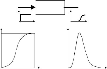
Constant infusion is conceptually similar to applying a step function to the system under study, while the output concentration curve is the step response of it. Many years later, the same Stewart came up with the sudden or single injection method, thereafter improved by W.F. Hamilton and his group, when they used a dye as indicator. This is equivalent to applying an impulse or Dirac function. Hence, the dilution concentration curve represents the impulse response of the system. As a consequence, the engineering student should not be surprised if the concentration output after constant infusion is proportional to the time integral of the concentration response after a single injection (Figure 2.9). One important requirement is a really fast injection of the indicator bolus, which obviously faces practical limitations. Quite interesting, too, is the fact that two engineers, C.M. Allen and E.A. Taylor, back in 1924, used

Constant infusion

F[mL/s] , I [mg/s]

Detection site

F

Figure 2.9. CONSTANT INFUSION METHOD TO OBTAIN FLOW. Saturation is reached at Cmax.

salt as a marker for water measurements in hydraulic systems (Grodins, 1962; Zierler, 1962, 1963).

Suggested exercises: Make a list of the possible limitations referred to above. Remember that the sudden single injection has the Dirac function as its ideal. Make also a list of the requirements needed for a good indicator. There is a compromise of two opposing and conflicting requirements. Is there a perfect indicator?

The indicator-dilution curve, as the single injection response of the hydraulic system under study, can be viewed from another reference frame. Say, now, that we are studying the time it takes to the particles of a population to traverse a hydraulic system when carried by a flow F, from the injection to the detection site (Figure 2.7). Even though they are transported by the same average flow, some will move faster than others. They are running some sort of race and the analogy is quite valid: All runners start at the same time, but those that run at higher speed will reach the detecting site sooner while most of them will get there later, while a smaller slower group will be last. A recording camera would