

Understanding the Human Machine - A Primer for Bioengineering - Max E. Valentinuzzi
.pdf68 |
Understanding the Human Machine |
Goldman–Hodgkin–Katz or GHK equation, which takes into account both permeabilities and ionic concentrations and, thus, can be applied at any moment of the action potential,
|
[K + ]i + PNa P |
[Na+ ]i |
|
|
Em = −61.5log10 |
K |
(2.57) |
||
[K + ]o + PNa P |
[Na+ ]o |
|||
|
|
|||
|
K |
|
||
It is illustrative to insert actual numbers into the equation in order to test it and see how the different components affect the membrane potential. A better exercise is to plot the membrane potential as a function of each parameter in the equation keeping the others at fixed values. Use any of the available programs (such as MathCad, Excel, or the like).
An excellent and more detailed account of the preceding paragraphs is to be found in the classic textbook by Ruch and Patton (1966). Through INTERNET, the student can have access to ELECTROPHYSIOLOGY OF THE NEURON (http://tonto.stanford.edu/eotn), a rather recent nice interactive tutorial, by John Huguenard (John.Huguenard@stanford.edu) and David A. McCormick (David.McCormick@Yale.edu). The authors are, respectively, with the Department of Neurology and Neurological Sciences at Stanford University School of Medicine, Stanford, CA, and with the Section of Neurobiology at Yale University School of Medicine, CT. More elaborate and rigorous demonstrations of Nernst equation can be found elsewhere in the literature, as for example in Plonsey’s classic book on bioelectric events (1969).
Two significant contributors to the subject were Frederick George Donnan (1870–1956), from the Physical Chemistry Laboratory at University College, London (Donnan, 1925–6), and Josiah Willard Gibbs (1839–1903), born in New Haven, Connecticut. The latter received from Yale University, in 1863, the first doctorate of engineering to be conferred in the United States. During a three-year stay in Europe, he received influence of high caliber scientists, such as Kirchhoff and Helmholtz (considered perhaps as the first biomedical engineer). He returned more a European than an American scientist in spirit, one of the reasons why general recognition in his native country came so slowly. In 1876 Gibbs published the first part of the work for which he is most famous, On the Equilibrium of Heterogeneous Substances, publishing the second part of this work in 1878. It is universally recognized that its publication was an event of the first importance in the history of chemistry.
− Propagation of the action potential
Excitability per se, as an electrical change, is just a local phenomenon, quite interesting and amazing, but of limited use for a living organism. The second characteristic that really enhances bioelectricity raising it to its full power is the propagation or conduction of the electrical change — the action potential — to adjacent parts of the excitable tissue. It is so
Chapter 2. Source: Physiological Systems and Levels |
69 |
that it can travel at high speeds to areas distant from the original stimulus, traversing complex networks, and eliciting all kind of responses essential for life.
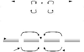
Once a given portion of an excitable fiber is fully depolarized to maximum activity (sign reversal), small potential gradients appear between the depolarized region and the yet resting neighbor areas to each direction, creating local current loops which depolarize them and, thus, generate new action potentials, one to the left and another to the right (Figure 2.22, upper part). This is the basic smooth conduction mechanism in nerves and muscles.
A discontinuous sheath of an electrically insulating fatlike substance called myelin, however, covers an important part of nerve fibers. It forms sleeves approximately 1 to 2 mm long and about 2 µm thick. In-between,
|
|
|
|
|
|
Excited part |
|
|
|
|
|
|
|||
|
|
|
|
|
|
|
|||||||||
|
|
|
|
|
|
|
|
|
|
|
|
|
|
|
|
|
+ + + + + + + + - - - - - - + + + + + + + + |
|
|
||||||||||||
|
|
- - - - - - - - - + + + + + - - - - - - - - - |
|
|
|||||||||||
|
|
|
|
Excitable fiber (nerve or muscle) |
|
||||||||||
|
|
|
|
|
|
Excited Node |
|
|
|
|
|
|
|||
Myelin |
|
|
+ |
|
|
|
|
|
|
|
|
|
|
|
|
|
|
|
|
|
|
|
|
|
|
|
|
|
|||
|
|
- |
|
+ |
|
|
|
|
|
||||||
sheath |
|
|
|
|
|
|
|
|
|||||||
|
|
|
|
|
|
|
|
|
|
|
|
|
|
||
|
|
|
- - - - |
+ + + + |
|
- - - - |
|
|
|
|
|||||
Node |
of |
Ranvier |
Intracellular fluid |
|
|
|
Local |
current loops |
|||||||
|
|
|
|||||||||||||
|
|
|
|
|
|
||||||||||
|
|
|
|
|
|
|
|
|
|
|
|
|
|
|
|
Figure 2.22. PROPAGATION OF THE ACTION POTENTIAL. Schematic representing a longitudinal section. Upper section - An excited portion acts as the stimulus to its adjacent right and left sections via the generation of depolarizing local current loops from positive to negative (curved arrows). This mechanism repeats itself to both sides resulting in the propagation of an action potential to the right and another to the left. By the time the two pulses reach their respective ends, the originally excited part is already recovered and ready to accept a second stimulus, if any. Lower section - It shows an important type of nerve fibers, covered by discontinuous sleeves of an insulating material called myelin. The cell membrane shows up only in-between, at 1µ gaps, the nodes of Ranvier. The local current loops only can be established between the excited one and the two immediate non-depolarized neighbors. Hence, there is some kind of jump (saltatory conduction).
70 |
Understanding the Human Machine |
the cell membrane shows up, at the nodes of Ranvier (after the French pathologist Louis Antoine Ranvier, 1835–1932). They are only 1µm wide. Hence, electrical charges concentrate around them, both outside and inside the cell. The electrical resistance across myelin is much higher than across the naked membrane (about 200 times). Conversely, the electrical capacitance across the membrane is about 200 times that across the sheath. Figure 2.22 (lower part) illustrates the conduction mechanism, similar to the one explained before, except that the current local loops “jump” or “leap” from node to node, for which reason it is named saltatory conduction. It has been demonstrated that a myelinated nerve can elicit a response only when the stimulus is applied to a node. If a node is blocked (as with cold or with an anesthetic), the local depolarizing loop can reach the next adjacent one and still propagate the action potential, but if two nodes are blocked, then propagation cannot proceed. The velocity of propagation greatly increases by the saltatory (jumping) trick. Quite an ingenious design!
Suggested exercise: There are several INTERNET Web Sites, entering for example with the word “Ranvier”, where more detailed explanations, even with animated images, very didactically illustrate both mechanisms of action potential conduction (smooth and saltatory). The student can also find names and places all over the world still active in the subject.
The velocity of conduction of the action potential, in any excitable tissue, is one aspect of concern with definite patho-physiological and clinical implications. Its measurement is based on the estimation of the time required for the action potential to traverse a known distance. Historically, it was first Hermann von Helmholtz (1821–1894) who, in 1850, in frog's sciatic nerve and using a rudimentary technology (a rheotome, a transformer and a galvanometer, very ingeniously arranged), reported a value of 30 m/s (Geddes and Hoff, 1968; Grüsser, 1997). Later on, in 1928, Erlanger and Gasser, both Nobel laureates, confirmed the value within 10% of error introducing in physiology with these measurements the oscilloscope and the electronic amplifier (Erlanger and Gasser, 1937). In whole muscles, it is now possible to estimate such velocity using certain properties of specific types of signal processing (Spinelli, Felice, Mayosky et al., 2001).
Suggested study subjects: Find out what a rheotome was. Analyze the etymology of the word. Search in the literature for the arrangement used by Helmholtz to measure conduction velocity.
Chapter 2. Source: Physiological Systems and Levels |
71 |
Analyze the direct approach used first by Helmholtz and, thereafter, by Erlanger and Gasser to measure the action potential propagation velocity. Study any of the indirect techniques based on signal processing and currently applied in electromyography to obtain the same parameter.
When reading this, think in terms of the evolution and development of concepts and in the influence of technology in physiology. The application of a new technology does not necessarily mean a new physiological concept.
After going over the preceding introductory electrophysiology concepts, it is suggested to read a series of four didactic articles in the subject written by Nassir H. Sabah (1999, 2000a, b, c).
− Electrophysiology of the heart
The myocardium is composed of bundles of myocytes (cardiac cells). Under the microscope, it shows striae (lines, bands) somehow reminding those seen in skeletal muscle, but really not quite because the bands are not as well organized and arranged as in the latter. Cardiac cells differ from skeletal myofibers in that cardiac myocytes have as a rule only one
1
2
0
3
4
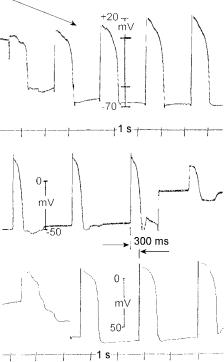
Figure 2.23. CARDIAC ACTION POTENTIALS. Upper record: A floating glass microelectrode pierced the cell membrane of a ventricular frog ventricle. Arrow above on the left indicates the piercing process, with a first beat when the electrode was on the surface, and a second beat with the electrode almost inside. The three last beats displays full action potentials. Diastolic potential was approximately – 70 mV with an overshoot of + 20 mV; thus, the total amplitude was 90 mV.
Lower two records: Two floating glass microelectrodes recorded simultaneously from the left atrium (above) and from the ventricle (below). The time difference of about 300 ms measures essentially the A-V delay. After the third beat (atrial channel) the electrode came off. The lowest record shows also penetration of the electrode on the left side. Records obtained by the author in 1967 at the Department of Physiology of Baylor College of Medicine.
72 |
Understanding the Human Machine |
nucleus per cell. Myocardial fibers are shorter than the fibers of skeletal muscle and rarely exceed 100µm in length, with a diameter in the order of 30µm–50µm. The shape is pretty irregular, showing projections to contact other cells in such a way that can be described as an anastomosing network. Such arrangement, very likely, tends to facilitate the propagation of the electric impulse.
The electrical phenomena associated with cardiac activity find their background in the general concepts of electrophysiology, but they show a number of peculiarities that have established cardiac electrophysiology as a specialty on its own. Any physiologist or biomedical engineer or physician can make a life in this important, attractive and fascinating field.
As any excitable tissue, all myocytes have a resting membrane potential and, when properly stimulated, trigger an action potential. Figure 2.23, shows atrial and ventricular action potentials recorded with microelectrodes. Hoffman and Cranefield (1960) published a superb and wellknown set of action potentials recorded from several cardiac fibers.
Roughly, these action potentials look like distorted rectangles and, in principle, can be (and have been) modeled by a rectangular pulse. The two nodes (S-A and A-V), however, deviate most from that model, displaying smooth rounded shapes. All show a depolarization upstroke (phase 0, a standardized denomination in cardiac electrophysiology, see Figure 2.23, atrial channel), from a minimum (the resting or diastolic membrane potential) to a maximum (the overshoot). The overshoot is not present in nodal fibers. The first and short repolarization return is usually called phase 1 (Figure 2.23, small spike). Many papers have been published to explain it; its study well belongs to the specialist and is beyond the boundaries of this textbook. The overshoot is followed by a plateau (phase 2), well marked in Purkinje and ventricular fibers and slowly falling off in atrial and His bundle fibers. It is as if the repolarization process were somewhat held on for a given time. Thereafter, repolarization speeds up (phase 3) until the membrane returns to the initial resting state (phase 4). The plateau is not shown by nodal fibers.
For the interested student, we suggest to visit the WEB entering with the words overshoot of the action potential. For example, Joe Patlak and Ray Gibbons (Department of Physiology, University of Vermont), in 1998 and 1999, offered simple and short accounts of the
Chapter 2. Source: Physiological Systems and Levels |
73 |
phenomenon without going into much details. The first microelectrode recordings from false tendons of dog hearts demonstrating the overshoot of the action potential upstroke were obtained by Coraboeuf and Weidman (1949). These are classic authors who produced substantial contributions to cardiac electrophysiology. This paper is written in French. We understand the difficulty, but the student should be aware that there is imporntant scientific literature written in languages other than English and that it would not hurt to learn how to read at least one foreign language (French, German, Italian, Russian, Portuguese or Spanish). Besides, it is fun. One extra language means another opened door.
Nerve and skeletal muscle action potentials are always short in duration, usually less than 1 ms. Cardiac action potentials, conversely, last between 200 and 400 ms, depending on the species and on the type of fiber. In other words, it is a very long metastable period. The duration of the contraction elicited by this action potential is of the same order of magnitude. In skeletal muscle, instead, a very short action potential triggers a longer contraction.
Study subject: Why cannot the heart enter into tetanic contraction? Do you know what tet-
Slow |
|
PCa ↑ |
|
|
Ca++ & Na+ |
|
PNa ↑ |
|
|
Inflow |
|
|
|
|
Depolarization |
|
|
|
|
PNa↑ |
PK ↓ |
Delay |
|
|
|
|
|
|
|
Na+ |
K+ |
PK ↑ |
PNa ↓ |
|
Influx ↑ |
|
|
|
|
Efflux ↓ |
|
|
|
|
|
|
K+ |
efflux ↑ |
Na+ influx ↓ |
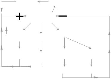
Figure 2.24. NOBLE’s ACTIVATION CYCLE. Compare this figure with Hodgkin’s activation cycle (Figure 2.21) for nerve and skeletal muscle. The long duration of the cardiac action potential is due to the effects of Ca++ and Na+ getting into the myocyte, but mainly to the former.
74 |
Understanding the Human Machine |
anic contraction is in skeletal muscle? Search in the literature for actual numerical values, say, comparing durations of action potentials and contractions in biceps or triceps with their counterparts in ventricular and atrial fibers of mammalian hearts. As a hint, check the following website: Medical Curriculum Objectives Project© 2001, The American Physiological Society (APS), Bethesda, MD.
Noble’s cycle
The activation process in heart cells is somewhat different than in either nerve or skeletal muscle. Figure 2.24 modifies Hodgkin’s cycle and summarizes the chain of events (Noble, 1962). Depolarization, after it is started, increases the permeability to sodium ions and simultaneously decreases the permeability to potassium. Due to the existing concentration gradients maintained by the sodium/potassium pump, an increment in Na+ influx and a decrement in K+ efflux take place, both events so reinforcing depolarization. Thus, a positive feedback loop is established leading to the fast depolarizing upstroke (phase 0). Slower Ca++ and Na+ channels due to increases in their respective permeabilities allow entrance of these ions into the cell and, hence, since they carry positive charges, depolarization is held on (plateau or phase 2). After some delay, the effect of depolarization on the permeabilities is reversed leading to the repolarization process in a braking negative loop. Explanation and interpretation of phase 1 are relatively controversial and, thus, should be left for more advanced courses in electrophysiology.
Noble did not consider these latter calcium and sodium channels in his first 1962 paper. They were reported years later, by McAllister, Noble and Tsien who developed a Purkinje fiber model in 1975 and which, thereafter, led to the Beeler–Reuter mammalian ventricular model in 1977. Many experiments were performed to provide a greater insight into the working of the ion channels in cardiac tissue. Finally, Di Francesco and Noble (1985) constructed a new and now well-recognized model of cardiac electrical activity. It is recommended to search in INTERNET entering with the words calcium and cardiac action potential. There are several didactic and even interactive proposals that the student can enjoy and profit from. Send a requesting message, for example, to info@cellml.org. The Department of Physiology of Loyola University Chicago (Maywood, IL 60153), in turn, has developed another model that incorporates many findings on cardiac calcium regulation and ionic currents (LabHEART, by J.L. Puglisi and D.M. Bers, 2001).
Figure 2.25 graphically describes the time course development of cardiac action potentials and the various permeability changes of the membrane associated with them (both, in the case of ventricular and S-A node fi-
Chapter 2. Source: Physiological Systems and Levels |
75 |
potentialMembrane |
ENa |
[mV] |
|
|
20 |
|
0 |
|
-80 |
|
EK |
PNa
and
PK
PCa
ENa
EK
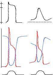
Figure 2.25 PERMEABILITIES AS TIME COURSE EVENTS. The upper portion displays action potentials of a ventricular fiber (left) and an S-A fiber (rigth), while the two lower lines show permeabilities to sodium (red), potasium (blue) and calcium (black), as they temporally correlate to each other. Sodium permeability opposes potassium’s, so reminding the behavior of a multivibrator collector potentials. Mainly after a course of Electrophysiology offered by Dr. Robert Vick, Department of Physiology, Baylor College of Medicine, Houston, TX, 1967.
bers). Action potentials are also bounded, above and below, by the potassium and sodium potentials (see Figure 2.19). Observe that, tipically, the potassium potential of a nodal fiber is always less negative than that of any other cardiac fiber. Such characteristic partially accounts for the instability of the nodal diastolic potential. The permeabilities to sodium and potassium change in opposite directions, reminding the behavior of a bistable multivibrator.
Partially summarizing: There are several types of cardiac fibers, showing histological and electrophysiological differences. In all likelihood, there are also differences in ionic concentrations. There might be differences too in their permeability rates of change. The four most significant ionic channels activated during the course of an action potential are, a rapid Na+ influx during phase 0, slow Ca++ and Na+ influx during the plateau phase 2, and slow K+ efflux during repolarization.
How did all this get started? Luigi Galvani, an Italian obstetrician, conducted in the city of Bologna a long series of experiments at the end of the 18th Century. They can be divided essentially in three kinds: With the first, he rediscovered the old phenomenon of electrostatic induction. Thus, there was no news. With the second, and by sheer serendipity, he found that the junction of a metal and an electrolytic solution could generate an electric potential to stimulate a frog’s muscle, but he never realized nor understood that and mistakenly thought he had found animal electricity. Unfortunately, he published a paper that was destroyed by Alessandro Volta, who developed further the idea and invented the elec-
76 |
Understanding the Human Machine |
tric pile, the first DC generator. In the midst of humiliation, poverty and family sorrow (for his wife had died), Galvani came up with a third experiment in frogs finally demonstrating the existence of animal electricity (now known as injury potential): When one portion of a sciatic nerve (still innervating its muscle, let us call it muscle 2) touched the injured part of another muscle (called, say, muscle 1) while a distant portion of the same nerve was held in contact with a normal uninjured portion of muscle 1, muscle 2 contracted. Obviously, the injury potential (negative inside and positive on the surface) acted as a stimulus during the “on” action. It was a manifestation of the membrane potential, recorded with microelectrodes 150 years later (in 1948), and the birth of modern electrophysiology. On the other hand, the strong controversy he maintained with Volta gave rise to the electric pile and, with it, to the beginning of current electricity (Hoff, 1936; Geddes and Hoff, 1971). Quite a couple of outstanding accomplishments.
2.2.2.2. Origin of the heart beat: the pacemaker
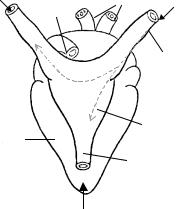
In herptiles (amphibia and reptilia), the heart has three stages and four chambers: the sinus venosus SV, two atria and one ventricle with the left and right side partially connected through the opening of an incomplete septum. Yes, there is some mixture of blood, but not too much due to the particular helicoidal configuration of this wall. Each stage has an electrical activity and the associated mechanical contraction. Hence, blood moves from the SV to the atria to the ventricles.
Left Ant. |
|
Aortas |
Right Ant. |
V. Cava |
Pulmon. |
||
|
|
V. Cava |
|
|
Vein |
|
|
|
|
|
|
|
122 |
7 |
|
|
|
Right |
|
|
86 |
34 |
|
|
pre-sinus |
||
|
65 |
|
|
|
|
67 |
|
|
122 |
|
Sinus V. |
Ventricle |
|
|
|
Post V.
Cava
Figure 2.26. FROG’s HEART. Posterior view. The sinus venosus SV has a triangular shape. It receives blood from the posterior vena cava (which brings blood from the lower body) and from the left and right venae cavae (returning blood from the upper portion of the body). The pacemaker is usually placed either at the right or at the left side of the upper SV, at the presinus area. From there, the electric impulse propagates to the other side and to the lower SV, to the atria atria and to the ventricles. Numbers show propagation times in ms measured from the origin. The frequency was 45/min.
Chapter 2. Source: Physiological Systems and Levels |
77 |
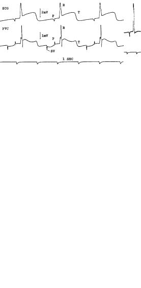
Figure 2.27. SINUS VENOSUS ELECTRICAL COMPLEX. Surface electrocardiogram recorded from an anesthetized snake (Elaphe obsoleta, the commonly called chicken snake in Texas) showing the SV activity followed by the atrial P wave, the ventricular QRS complex and an inverted T wave. Time marks are 1 s apart. The vertical bar by the third beat corresponds to a calibration of 1 mV. Record obtained by the author.
The sinus venosus SV has a triangular shape (Figure 2.26); it receives blood from the posterior vena cava (which brings it from the lower body circulatory system) and from the left and right venae cavae (returning it from the upper portion of the body). The pacemaker is usually placed either at the right or at the left side of the upper SV, at the so-called presinus area. It is a natural oscillator (marking the heart pace or rhythm), with an unstable resting potential (called diastolic potential). From there, the electric impulse propagates to the other side and to the lower SV, to the atria and to the ventricles.
The snake is a particular good model to record the electrical and mechanical activities of its heart (Valentinuzzi, 1969). Figure 2.27 displays
Figure 2.28. SINUS VENOSUS ELECTRICAL COMPLEX AND OTHER COMPONENTS. From an anesthetized snake (Elaphe obsoleta). The upper channel is a surface ECG while the lower channel was obtained with a bipolar catheter in the sinus venosus introduced via the posterior vena cava. The sequence is clear: SV, P, R and T. The elevation of the S-T segment in both channels indicates some ventricular damage. After Valentinuzzi and Hoff (1970).