Understanding the Human Machine - A Primer for Bioengineering - Max E. Valentinuzzi

show this phenomenon very clearly. Well, the dilution curve at the detecting site is some kind of “recording camera”: the early arrival times are obviously made by a few, then there is a sharp increase until a maximum is reached (most of the particles arrive at time tmax), and thereafter and asymmetrically, less and less particles get to the detecting site (these are the slow ones). Thus, the dilution curve can be interpreted also as the only continuously recorded event that yields the distribution of arrival times, at a given site, after introduction of a known number of particles in an upstream injecting place. It can be demonstrated that it follows the so called Poisson distribution (Figure 2.8).

Cardiac output measurement, in general, and the overall theory and practice of the indicator-dilution method is a wonderful chapter of hemodynamics and hydraulics, highly attractive to the engineering student, with aspects still deserving attention and calling for further development.

− Cerebral and coronary flows

Knowledge of the overall and average blood flow to the brain and myocardial mass is obviously very valuable. They are the most important beds. One drawback, though, is that this value does not supply information regarding the distribution of blood throughout the region, for some areas may not be well perfused leading to tissue damage.

Blood gets to the brain via the two carotid arteries (easily felt by finger palpation on the neck, at both sides of the trachea) and, to a lesser degree, via the two vertebral arteries, on the back of the neck. Return takes place through veins that run parallel to the above-mentioned arteries. Kety and Schmidt developed a method, in 1948, for the measurement of the average blood flow to the brain per unit of tissue mass.

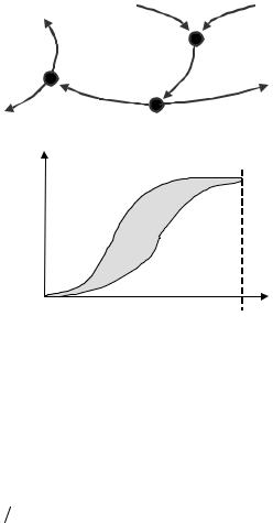
Let us draw a flow diagram (Figure 2.10) with three nodes: the lungs, L, the left ventricle, LV, and the cerebral mass, M. We also have a patient breathing nitrous oxide, N2O, at a rate of N [mL/min]. The patient will fall into sleep because this gas is anesthetic, traversing very easily the tissue barriers. There is a total flow of blood, F, to the lungs from the right heart and from the lungs to the left ventricle. From the latter, the greatest portion proceeds to the general circulation, while a small fraction, Fcer [grams blood/min], supplies the brain. This is precisely the regional flow we are interested in. It carries a high concentration, A(t) [mL gas/gram blood] and, as it perfuses the brain, it diffuses through the capillary walls, the interstitial space and the nervous cell membranes getting into the intracellular space. Thus, the brain tissue takes up nitrous oxide

A(t)

V(ts) = Vu

Area

V(t)

Time

Figure 2.10. NODE SYSTEM TO OBTAIN THE CORONARY OR THE CEREBRAL BLOOD FLOW. It must be underlined that only an average value per unit mass of tissue is obtained.

at a rate dQb/dt, measured in [mL gas/min]. Evidently, the venous blood outflow will carry a low gas concentration, V(t), because there was tissue extraction. At the node M, the continuity principle states that, at dynamic equilibrium conditions, the amount of gas that goes in must be equal to the amount that goes out. In mathematical terms, it writes,

where, we repeat, there are flow of blood in [g bl/min], flow of N2O in [mL gas/min], and concentration of gas in [mL gas/g bl]. The student should practice with the units to fully grasp the concept. This is why there is some repetition, precisely to underline its importance.

From eq. (2.23), it is seen that the nitrous oxide uptake rate appears as,

where A and V are functions of time obtained experimentally (Figure 2.10) sampling and testing blood for gas content at regular intervals. Both curves tend approximately to the same saturation level, with venous blood concentration staying always slightly below arterial concentration.

The total gas amount taken up by the brain is the integral, between the initial and the saturation time, Ts, of the latter equation, so that, after solving for Fcer, it becomes,

where the denominator describes the shaded area depicted in Figure 2.10. Tracking down the units once more, it is seen that Qb has to be measured in mL of gas, thus well checking with the concentration and time units below in order to yield grams of blood per minute. The area is graphically calculated from the experimental records since arterial and venous samples (the latter from the jugular) are relatively easy to obtain, but there is no way of measuring or even estimating the total amount of gas absorbed by the brain. However, if eq. (2.25) is divided through by the weight W of the brain (of course, unknown), we get,

an expression still looking unusable. Hence, some more assumptions are needed.

Once the patient has breathed for a while (Ts = 10 to 15 s), the arterial and venous curves reach saturation and it is said that the gas concentration in brain tissue is in equilibrium with the gas concentration in venous blood, or

so describing a usual situation in exchangers in general. Moreover, it is also assumed that 1g blood is approximately equal to 1g tissue, which does not sound to bad because the density of lean tissue is about 1.10, that of fat tissue is around 1.03, and that of blood is between 1.05 and 1.06. Hence, considering (2.27), eq. (2.26) becomes simply,

where BF represents the brain flow expressed in g or mL of blood per min per g of tissue. Sometimes, a factor α (called the partition coefficient) is included in eq. (2.28) to account for the imperfect passage of substance across the tissue barrier. This factor is about 0.98–0.99 and has to be experimentally estimated. With this ingenuous procedure, the authors mentioned above reported, from 14 patients, an average flow of 54 mL/min for each 100 g of brain tissue, with a standard deviation of 12.

Exercise: First, compare eq. (2.22) with (2.25). Do you notice any similarity?

Derive now the expression for the coronary flow using the same approach as for the cerebral blood flow. Search for the necessary information. Where would you take the blood samples from? Average value is 78 g blood/min (or 73 mL bl/min) per 100 g of myocardium. Find out the approximate myocardial weight of an adult normal heart and calculate its total coronary flow. What percentage is it of the total flow? Brain and heart show also a remarkable autoregulation: search for more informartion about it.

There are techniques (as for example with radioactive microspheres or with technecium99 or tallium201, using the so called Single Photon Emission Computed Tomography, or SPECT) to estimate regional flows, both in the brain and the heart, so permitting a better evaluation of possible injuries and also of therapeutic strategies. It is, indeed, a highly specialized subject. The student is encouraged to search in the literature.

2.2.1.8. The pressure-volume loops

− Origins

Nicolas Léonard Sadi Carnot (1796–1832) was a French physicist and engineer who, in 1824, published a little and yet seminal contribution to science and technology: Reflexions sur la puissance motrice du feu et sur les machines propres a developer cette puissance (Thoughts about the power of fire and about the proper engines to develop such power). It was the foundational hallmark of thermodynamics, indeed, essential for the understanding and design of the internal combustion machines (such as the steam, gasoline and Diesel engines). In them, the pressure and volume handled by the cylinders with movable pistons which, in the end, transmit the force to produce the rotation of a shaft, give rise to the so called pressure-volume diagrams or loops.

Theoretical and practical thermodynamics developed rapidly all through the XIXth Century. Cardiac physiology, in turn, made significant progress. It was Otto Frank, in Germany in 1899, the first to bring the concept of pressure-volume loop into physiology, when with very rudimentary means he produced such a diagram from a frog’s ventricle. However, in the 1970's and 1980's, the group of the late Kiichi Sagawa, at Johns Hopkins University, after a careful and long series of studies, put this engineering concept in its adequate place and interpreted it within the overall frame of cardiac physiology, opening with it a complementary new and fresh vision (Sagawa, Maughan, Suga et al., 1988).

− Generation and description of a PV-loop

Electronics Engineering students are familiar with the Lissajous figures. They are predictable nice looking composite patterns obtained by combining two sinusoidal signals injected, simultaneously and respectively, to the x-horizontal and y-vertical plates of an oscilloscope after disconnecting the horizontal internal sweep. The pressure-volume diagrams are some sort of Lissajous patterns except that the component signals, while still periodic, are not sinusoidal. One is the intraventricular pressure, Piv, and the other, the intraventricular volume, Viv, both as time course events experimentally obtained. In fact, any of the four cardiac chambers can produce such a loop.

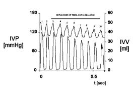
Figure 2.11 displays ten beats recorded from an experimental dog. The upper channel is the left intraventricular volume, calibrated in milliliters and detected by a set of electrodes which measure blood conductance within the chamber (conductance is proportional to volume), while the lower channel is the left intraventricular pressure, calibrated in mmHg and detected by a miniature transducer, also placed within the chamber.

For each beat, volume, as time proceeds, shows a downstroke from a maximum value (end diastolic volume) to a minimum level (end systolic volume), thus, describing ejection. Thereafter, it is followed by a rising limb back to a peak value and, hence, marking the filling phase of the left ventricle. Observe that the ventricle never empties completely. Pressure, instead, always starts from zero (or almost zero) abruptly climbing to the maximum value and displaying a rectangular-like shape.

As an exercise, the student should take a careful look at these records trying to correlate them in time.

Figure 2.12 combines beats 2 and 3 shown in the preceding Figure 2.11

Figure 2.11. INTRAVENTRICULAR VOLUME AND PRESSURE RECORDS. They are displayed as time course events during a preload maneuver. Volume above (calibration on the right side) and pressure below (calibration on the left). Obtained at the Departement of Bioengineering, UNT, 1995.

C B

D A

END SYSTOLIC VOLUME STROKE VOLUME

Figure 2.12. INTRAVENTRICULAR VOLUME-PRESSURE DIAGRAMS. Beats 2 & 3 of the previous Figure 2.11 were combined as orthogonal signals producing a Lissa- jous-like pattern, that is, two almost coincident PV-loops. The two isovolumetric phases (relaxation, on the left, and contraction, on the right) take place along the levels, respectively, of the end-systolic volume, and of the end-systolic volume plus stroke volume = end-diastolic volume. Points A and C mark the beginning and end of the mechanical systole (subdivided in the isometric contraction and ejection phases). The vertical arrow on the right shows the counter-clockwise rotation of each beat. On its way back to A, the cycle enters into its diastolic portion (subdivided, in turn, into relaxation and mainly passive ventricular filling, the latter from D to A). The four corners correspond to the openings and closures of both left cardiac valves.

to yield the Lissajous-like shape of two typical PV loops, both almost coincident. Roughly, the corners of this quasi-quadrangular figure identify the four characteristic points of the cardiac cycle. They signal the openings and closures of the cardiac valves: A(Ved, Ped), defined by the end-diastolic volume and pressure, respectively; B(Ved, Pop), defined by the same end-diastolic volume and a much higher pressure than the preceding one, which can be called the opening pressure because it is larger than the aortic pressure and, thus, it opens the aortic valve, so starting the ejection phase. Ventricular contraction started at A, which coincides with the closure of the mitral valve (for the intraventricular pressure becomes higher than left intra-atrial pressure), intraventricular pressure rises to Pop and that contraction keeps on going sustaining pressure during all ejection until the pressure inside the chamber falls below the aortic level triggering the closure of the aortic valve. That is point C(Ves,, Pes), defined by the end-systolic volume and pressure, respectively. The same point marks the end of ventricular mechanical systole, as point A characterizes its beginning.

Thereafter, the myocardium relaxes isovolumetrically (at constant volume) at a fast decreasing pressure, until it reaches zero or almost zero, when the low but higher left intra-atrial pressure opens the mitral atrioventricular valve. It is point D(Ves, Po), defined by the previous endsystolic volume and an almost zero intraventricular pressure, and signaling the beginning of ventricular filling phase, which ends at A, to start all over again in the next beat. Hence, the whole cardiac cycle is divided in two halves: systole, between A and C (closure of the mitral valve and of the aortic valve), and diastole, between C and A (closure of the aortic valve and of the mitral valve). Each semicycle is, in turn, subdivided in two phases: First, the isovolumetric contraction of the ventricle, between A and B, that is, when both valves are closed and, thus, the chamber cannot change its volume (blood is essentially incompressible). Most of the energy consumption takes place during that short phase. Second, the already introduced ejection phase, between B and C, when the aortic valve is fully opened and blood is propelled into the elastic aortic reservoir. Finally, at diastole, we find the isovolumetric relaxation, between C and D, and the last filling phase.

Exercise: Compute the area encompassed by one of the two loops shown in Figure 2.12 using any means you may have at hand. How would you interpret it? Give a thought to the units.

Question: By what mechanism cardiac valves open and close?

− The FSSS line

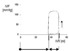
Figure 2.13 displays eight loops after composing eight pressure and volume beats, both as time course events, during inflation of an intra-caval balloon, as indicated in Figure 2.11 (upper continuous bar). This is called in the hemodynamics jargon a preload maneuver. Transient occlusion of that great vessel (10 to 30 s, at the most) significantly reduces the venous return to the left atrium, in turn reducing the amount of blood to the left ventricle. According to Starling's Law, a reduction both in pressure and stroke volume must be expected, as clearly shown in the temporal records. The manifestation of such phenomenon in the PV-plane is a sliding of the loops to the left, with the end-systolic point (C point) describing a straight line which is called the Frank–Starling–Suga–Sagawa (or FSSS) line. It has been demonstrated that that line (essentially its slope) can be used as an estimator of the contractility of the myocardium, or, in other words, as a measure of the myocardium inotropic condition. A lin-

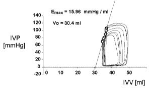
Figure 2.13. END-SYSTOLIC LINE (or Frank–Starling–Suga–Sagawa Line). It was obtained with a preload maneuver, that is, a partial occlusion of the venous return to the right heart, producing a shift to the left and downward of the PV loops. The latter behaved as “if hanging from the line and sliding down”. See text for details. Obtained from a patient at the Institute of Cardiology of Tucumán with the technical assistance of the Department of Bioengineering, UNT, 1996.

ear regression of the end-systolic points obtained by a preload maneuver produces an equation of the type,

where Emax stands for its slope, and Vo , for the horizontal axis intercept. There has been considerable discussion over the detailed definition of the C points on the loops and over the meaning of the volume for zero pressure. One relatively well accepted stance is that the end-systolic point occurs where the absolute slope of the PV-loop is maximum, i.e., when P/V reaches a maximum. However, the Emax is a statistical value obtained from the collection of perhaps eight to ten such maximum slope data points in a single maneuver. When pressure is zero, there is a residual volume which Sagawa and collaborators named the dead volume. Much has been written regarding its interpretation. It shows wide spread and its true meaning still remains controversial, especially when now and then some negative values come up.

The filling phase of the cardiac cycle corresponds to the passive increase in pressure as volume is steadily increased in a balloon, an experiment easily carried out in any lab. If one measures the increments ∆V, with a calibrated syringe, and simultaneously one reads the resulting increments ∆P, with a manometer, the overall passive PV-relationship can be plot-

ted, so graphically describing the elastic properties of the material. Under ideal conditions, it is linear, following the well-known Hooke's Law, i.e.,

from which, by differentiation, one gets dP/dV = k, the elastance of the material, obviously the inverse of the compliance, as already introduced above.

Suggested exercise: First, check in any physics textbook for the regular statement of Hooke's Law, as applied, for example, to a string under tension. Play mathematically with it to obtain eq. (2.30). Equation (2.29) has the same mathematical form, with its slope being also an elastance. However, does it describe a passive or an active parameter?

Let us underline that during a preload maneuver, the PV-loops shift progressively to the left, with the end-systolic points sliding down the FSSS line, as if “hanging” from a cable. The base, that is, the filling phase DA, also slides to the left and slightly downward, following the passive elastic PV-relationship. Such relationship, however, is not linear, being usually approximated by an exponential function. Thus, the latter acts as some sort of lower rail. An inflatable balloon can also be inserted in the thoracic aorta via, say, one of the femoral arteries. During inflation for a few seconds, it tends to hinder the outflow of blood from the left ventricle leading to an increase in intraventriculer pressure and a transient accumulation of blood in it. This is called an afterload maneuver. The PVloops shift upward and to the right, but always “hanging” from the FSSS line and sliding over the passive non-linear PV-relationship (Valentinuzzi & Spinelli, 1989; Feldman, Erikson, Mao et al., 2000; White, Brookes, Ravn et al., 2001; de Vroomen, Steendijk, Lopes Cardozo et al., 2001). In normal physiological conditions, the heart moves constantly in this fashion, adjusting itself almost beat by beat to the demands. Even more, certain substances (as for example, epinephrine, in the case of exercising) can modify the position of the FSSS line (steeper slope) and, hence, offering more room for the left ventricle to operate. Everything that has been said so far for the left ventricle is also applicable to the right, keeping in mind the lower pressure it works with. An ischemic ventricle, instead, will contract with less force and the line would drop (lower slope). See the references given above in this same paragraph to illustrate.

Review exercise: Using published records found in the literature, draw by hand a left ventricular PV-diagram marking and identifying the four characteristic points. Do the same for the right ventricle. Identify the valves you are dealing with.

Jules Antoine Lissajous (1822–1880) was a French physicist who studied at the École Normale Supérieure, in Paris. His doctoral dissertation, in 1850, was devoted to the recordings of vibrations. In 1873, he was awarded the Lacaze Prize. The theoretical analysis of his famous patterns can be found in any physics textbook (for example, Page, 1965) under the heading of simple armonic motion.

Sadi Carnot graduated from the École Polytechnique, in Paris in 1814. He worked on the mathematical theory of heat and helped start the modern theory of thermodynamics. In 1824, he published the only work during his lifetime that includes his description of the ideal cycle. This work became well known after Clapeyron published an analytic reformulation in 1834. It was incorporated into the thermodynamic theory of Clausius and Thomson. It is not known whether Otto Frank was directly influenced by these physics and engineering concepts. In his papers there is no reference to them but, as a well-informed high-level scientist, he must have been aware of that knowledge.

2.2.1.9. Arterial input impedance

− Definition: First component

Two terminals of a given circuit will tend to oppose to a change of state when an excitation is applied. If the latter is a sinusoidal voltage, V, the system will present some hindrance to the establishment of a sinusoidal current, I. The relationship of V to I, in the s-domain, and only in the s- domain, as a generalization of Ohms' Law, gives the simplest mathematical definition of the electrical impedance of the system. All electrical engineering students and practitioners are well familiar with this concept. Thus,

where the impedance Z is, obviously, a complex function of the complex frequency s.

A similar rationale can be used in the vascular tree: Vascular impedance expresses the relation of the forces acting in the bloodstream to the resulting motion of blood (Milnor, 1982). The physical properties of the blood and of the blood vessels determine vascular impedance. Therefore, it contains information of paramount importance. The concept was first introduced by J.R. Womersley, in 1955, furthered by his close associate D.A. McDonald, in 1955 and subsequent years and, later on, more elaborated by other authors, like Patel, Greenfield & Fry (1964). Milnor's classic book referred to above lists all the significant literature up to that year. The concept is valid for the aorta, the pulmonary artery, arteries supplying specific beds (like the kidneys, the liver, the legs, or any other), or just any vessel, including veins.