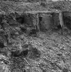
Fig. 4.7. The Opalinus Clay in the Siblingen clay pit, Switzerland. Note the marked planar jointing (image courtesy of Nagra).

provides access to the rock mass on a larger scale than is possible in boreholes and allows better correlations to be developed between boreholes. Where exposure is limited, maximum use should therefore be made of man-made structures such as quarries, brick pits, etc., combined, where appropriate, with other survey methods, such as aerial geophysical techniques, geochemical mapping, multiple shallow boreholes, etc.

Where possible, access to the underground should be sought in tunnels, mines, etc. Such structures, even if they are at considerably shallower depths than is expected for a repository, can provide useful information on the larger scale on geological structures, groundwater flow, etc., especially if records of tunnelling are examined, as is indicated above. Great care has to be taken, however, when the only sources of data are shallow tunnels and boreholes (e.g., JNC, 2000) as this can clearly produce a biased database which may not reflect the rock properties at repository depth (cf. the example above of the Opalinus Clay). This can lead to very pessimistic assumptions on the likely qualities of the repository host rock, possibly leading to ‘‘over-engineering’’ of the EBS in later assessments.

4.2.2.1. Hydrogeology

To understand the groundwater flow system in and around the site under investigation, it will be necessary to study the hydraulic properties of the formations and the distribution of hydraulic heads, possibly over a large area. The geological investigations will provide the structure of the site and the lithological distributions, from which a hydrogeological model, or models, can begin to be developed (e.g., Fig. 4.8, which illustrates the link between the stratigraphy, lithology and the way in which the rock types are represented in the groundwater flow models). It is likely that this modelling will be carried out on different scales, from the regional to the local or site scale.

of 300 km2 and with boundary conditions determined from the larger-scale models (Fig. 4.10). This model was used as the basis for calculating the migration/dispersion of radionuclides from the repository and needed to have the required degree of detail and be as limited as possible geographically in order to avoid excessive calculation times.

As well as developing an understanding of the groundwater flow system, it is also important, perhaps of greater importance, to develop an understanding of the hydrochemical system – to determine the composition of the groundwaters, to relate these compositions to the mineralogy of the rocks and to determine the chemical evolution of the groundwater system over long periods of time. Geochemical work has two important advantages over purely hydrogeological investigations; one of these is that historical data can be extracted directly from geochemical studies without the uncertainties associated with the long-term extrapolation of groundwater flow models and the second is that a large number of variables can be measured. Most natural systems are likely to provide in excess of 250 constituents which could be measured, each of which will provide some information on one or more pieces of the overall picture, such as the residence time of the groundwater, its chemical characteristics at the time of recharge, the chemical reactions that have taken place, the extent of mixing of different groundwater systems, etc.

The sampling and analysis of groundwater from boreholes forms an essential element in a site investigation and, to ensure the collection of representative samples, the sampling programme must be included in the initial design of the borehole programme. While it is comparatively easy to obtain high-quality groundwater samples in aquifers using sampling systems that preserve the in situ pressure of the groundwater at the sampling depth, it is considerably more difficult to obtain such samples in clays (or any other very low-permeability formations such as an evaporite). In such rocks, the inflow of groundwater into any sampling system is likely to be extremely small and recourse may have to be made to pore fluid extraction from clay samples in the laboratory, by techniques such as squeezing, or by other techniques in the case of evaporites. Extensive work has been carried out over the last decade on the physico-chemical processes in deep clays, as they have become of greater interest for the disposal of radioactive waste, and chemical studies do provide one of the best methods of demonstrating the processes that have taken place in such clays over long periods of time – perhaps as much as several million years (e.g., Nagra, 2002a; ONDRAF, 2001a,b). Similarly, it is possible to demonstrate the slow rates of chemical change that have taken place in evaporites.

Figure 4.11, for example, shows the 2H profile through the Opalinus Clay, which lies between two more permeable formations of the Malm and the Keuper, and a similar profile exists for chloride and other elements. The measured values have been compared with the results of a pure diffusion model and the good fit demonstrates that there is no significant vertical advective flow. The value of such data, which is equivalent to a longterm, natural experiment, is that the results are relevant for long timescales (in this case perhaps as much as many millions of years) and over significant distances (again in this case more than 100 m). Similar results in other clays at depth could also indicate similar times and distances. Data of this type therefore provide convincing evidence of the stability of this type of natural system at depth – something that is of considerable advantage in being able to demonstrate the intrinsic suitability of such an environment for disposal purposes.