

1manly_b_f_j_statistics_for_environmental_science_and_managem
.pdf66 Statistics for Environmental Science and Management, Second Edition
The mean and variance of a continuous distribution are the sample mean and variance that would be obtained for a very large random sample from the distribution. In calculus notation, the mean is
µ = ∫ x f (x)dx
where the range of integration is the possible values for the x. This is also sometimes called the expected value of the random variable X, and denoted E(X). Similarly, the variance is
σ2 = ∫ (x −µ)2 f (x)dx |
(3.11) |
where, again, the integration is over the possible values of x.
The continuous distributions that are described here are ones that often occur in environmental and other applications of statistics. See Johnson and Kotz (1970a, 1970b) for details about many more continuous distributions.
3.3.1 The Exponential Distribution
The probability density function for the exponential distribution with mean μ is
f(x) = (1/μ) exp(−x/μ), for x ≥ 0 |
(3.12) |
which has the form shown in Figure 3.3. For this distribution, the standard deviation is always equal to the mean μ.
f(x)
1.0
0.8
0.6
0.4
0.2
0.0
0 |
5 |
10 |
15 |
20 |
|
|
x |
|
|
|
Mean = 1 |
Mean = 2 |
Mean = 5 |
|
Figure 3.3
Examples of probability density functions for exponential distributions.
Models for Data |
67 |
The main application is as a model for the time until a certain event occurs, such as the failure time of an item being tested, the time between the reporting of cases of a rare disease, etc.
3.3.2 The Normal or Gaussian Distribution
The normal or Gaussian distribution with a mean of μ and a standard deviation of σ has the probability density function
f(x) = [1/√(2πσ2)] exp[−(x − μ)2/(2σ2)], for −∞ < x < +∞. |
(3.13) |
This distribution is discussed in Section A1.2 of Appendix 1, and the form of the probability density function is illustrated in Figure A1.1.
The normal distribution is the default that is often assumed for a distribution that is known to have a symmetric bell-shaped form, at least roughly. It is commonly observed for biological measurements such as the height of humans, and it can be shown theoretically (through something called the central limit theorem) that the normal distribution will tend to result whenever the variable being considered consists of a sum of contributions from a number of other distributions. In particular, mean values, totals, and proportions from simple random samples will often be approximately normally distributed, which is the basis for the approximate confidence intervals for population parameters that have been described in Chapter 2.
3.3.3 The Lognormal Distribution
It is a characteristic of the distribution of many environmental variables that they are not symmetric like the normal distribution. Instead, there are many fairly small values and occasional extremely large values. This can be seen, for example, in the measurements of PCB concentrations that are shown in Table 2.3.
With many measurements, only positive values can occur, and it turns out that the logarithm of the measurements has a normal distribution, at least approximately. In that case, the distribution of the original measurements can be assumed to be a lognormal distribution, with probability density function
f(x) = {1/[x√(2πσ2)]} exp{−[loge(x) − μ]2/(2σ2)}, for x > 0 |
(3.14) |
Here μ and σ are, respectively, the mean and standard deviation of the natural logarithm of the original measurement. The mean and variance of the original measurements are
E(X) = exp(μ + ½σ2) |
(3.15) |
and |
|
Var(X) = exp(2μ + σ2)[exp(σ2) – 1] |
(3.16) |

68 Statistics for Environmental Science and Management, Second Edition
f(x)
1.8
1.6
1.4
1.2
1.0
0.8
0.6
0.4
0.2
0.0
0 |
1 |
2 |
3 |
4 |
|
|
x |
|
|
|
Mean = 1, SD = 0.5 |
Mean = 1, SD = 1 |
Mean = 1, SD = 2 |
|
Figure 3.4
Examples of lognormal distributions with a mean of 1.0 and standard deviations of 0.5, 1.0, and 2.0.
Figure 3.4 shows some examples of probability density functions for three lognormal distributions.
3.4 The Linear Regression Model
Linear regression is one of the most frequently used statistical tools. Its purpose is to relate the values of a single variable Y to one or more other variables X1, X2, …, Xp in an attempt to account for the variation in Y in terms of variation in the other variables. With only one other variable, this is often referred to as simple linear regression.
The usual situation is that the data available consist of n observations y1, y2, …, yn for the dependent variable Y, with corresponding values for the X variables. The model assumed is
y = β0 + β1x1 + β2x2 + … + βpxp + ε |
(3.17) |
where ε is a random error with a mean of zero and a constant standard deviation σ. The model is estimated by finding the coefficients of the X values that make the error sum of squares as small as possible. In other words, if the estimated equation is
yˆ = b0 + b1x1 + b2x2 + … + bpxp |
(3.18) |
then the b values are chosen so as to minimize the sum of squares for error
SSE = Σ(yi − yˆi)² |
(3.19) |

Models for Data |
69 |
where the yˆi is the value given by the fitted equation that corresponds to the data value yi, and the sum is over the n data values. Statistical packages or spreadsheets are readily available to do these calculations.
There are various ways that the usefulness of a fitted regression equation can be assessed. One involves partitioning the variation observed in the Y values into parts that can be accounted for by the X values, and a part (SSE, above) that cannot be accounted for. To this end, the total variation in the Y values is measured by the total sum of squares
SST = Σ(yi − y)2 |
(3.20) |
This is partitioned into the sum of squares for error (SSE) and the sum of squares accounted for by the regression (SSR), so that
SST = SSR + SSE
The proportion of the variation in Y accounted for by the regression equation is then the coefficient of multiple determination,
R2 = SSR/SST = 1 − SSE/SST |
(3.21) |
which is a good indication of the effectiveness of the regression.
There are a variety of inference procedures that can be applied in the multiple regression situation when the regression errors ε are assumed to be independent random variables from a normal distribution with a mean of zero and constant variance σ2. A test for whether the fitted equation accounts for a significant proportion of the total variation in Y can be based on Table 3.1, which is called an analysis-of-variance table because it compares the observed variation in Y accounted for by the fitted equation with the variation due to random errors. From this table, the F-ratio,
F = MSR/MSE = (SSR/p)/[SSE/(n − p − 1)] |
(3.22) |
can be tested against the F-distribution with p and n − p − 1 degrees of freedom (df) to see if it is significantly large. If this is the case, then there is evidence that Y is related to at least one of the X variables.
Table 3.1
Analysis-of-Variance Table for a Multiple Regression Analysis
Source of |
|
Degrees of |
|
|
Variation |
Sum of Squares |
Freedom (df) |
Mean Square |
F-Ratio |
|
|
|
|
|
Regression |
SSR |
p |
MSR |
MSR/MSE |
Error |
SSE |
n – p – 1 |
MSE |
|
|
|
|
|
|
Total |
SST |
n – 1 |
|
|
|
|
|
|
|

70 Statistics for Environmental Science and Management, Second Edition
The estimated regression coefficients can also be tested individually to see whether they are significantly different from zero. If this is not the case for one of these coefficients, then there is no evidence that Y is related to the X variable concerned. The test for whether βj is significantly different from zero involves calculating the statistic bj/SÊ(bj), where SÊ(bj) is the estimated standard error of bj, which should be output by the computer program used to fit the regression equation. This statistic can then be compared with the percentage points of the t-distribution with n − p − 1 df. If bj/SÊ(bj) is significantly different from zero, then there is evidence that βj is not equal to zero. In addition, if the accuracy of the estimate bj is to be assessed, then this can
be done by calculating a 95% confidence interval for βj as bj ± t5%,n−p−1 bj/SÊ(bj), where t5%,n−p−1 is the absolute value that is exceeded with probability 0.05 for
the t-distribution with n − p − 1 df.
There is sometimes value in considering the variation in Y that is accounted for by a variable Xj when this is included in the regression after some of the other variables are already in. Thus if the variables X1 to Xp are in the order of their importance, then it is useful to successively fit regressions relating Y to X1, Y to X1 and X2, and so on up to Y related to all the X variables. The variation in Y accounted for by Xj after allowing for the effects of the variables X1 to Xj−1 is then given by the extra sum of squares accounted for by adding Xj to the model.
To be more precise, let SSR(X1, X2, …, Xj) denote the regression sum of squares with variables X1 to Xj in the equation. Then the extra sum of squares accounted for by Xj on top of X1 to Xj−1 is
SSR(Xj •X1, X2, …, Xj−1) = SSR(X1, X2, …, Xj) − SSR(X1, X2, …, Xj−1). (3.23)
On this basis, the sequential sums of squares shown in Table 3.2 can be calculated. In this table, the mean squares are the sums of squares divided by their degrees of freedom, and the F-ratios are the mean squares divided by the error mean square. A test for the variable Xj being significantly related
Table 3.2
Analysis-of-Variance Table for the Extra Sums of Squares Accounted for by Variables as They Are Added into a Multiple Regression Model One by One
Source of |
|
Degrees of |
|
|
Variation |
Sum of Squares |
Freedom (df) |
Mean Square |
F-Ratio |
|
|
|
|
|
X1 |
SSR(X1) |
1 |
MSR(X1) |
F(X1) |
X2|X1 |
SSR(X2|X1) |
1 |
MSR(X2|X1) |
F(X2|X1) |
. |
. |
. |
|
|
. |
. |
. |
|
|
Xp|X1, …, Xp–1 |
SSR(Xp|X1, …, Xp–1) |
1 |
MSR(Xp|X1, …, Xp–1) |
F(Xp|X1, …, Xp–1) |
Error |
SSE |
n – p – 1 |
MSE |
|
|
|
|
|
|
Total |
SST |
n – 1 |
|
|
|
|
|
|
|
Models for Data |
71 |
to Y, after allowing for the effects of the variables X1 to Xj−1, involves seeing whether the corresponding F-ratio is significantly large in comparison to the F-distribution with 1 and n − p − 1 df.
If the X variables are uncorrelated, then the F-ratios indicated in Table 3.2 will be the same irrespective of what order the variables are entered into the regression. However, usually the X variables are correlated, and the order may be of crucial importance. This merely reflects the fact that, with correlated X variables, it is generally only possible to talk about the relationship between Y and Xj in terms of which of the other X variables are in the equation at the same time.
This has been a very brief introduction to the uses of multiple regression. It is a tool that is used for a number of applications later in this book. For a more detailed discussion, see one of the many books devoted to this topic (e.g., Kutner et al. 2004). Some further aspects of the use of this method are also considered in the following example.
Example 3.1: Chlorophyll-a in Lakes
The data for this example are part of a larger data set originally published by Smith and Shapiro (1981) and also discussed by Dominici et al. (1997). The original data set contains 74 cases, where each case consists of observations on the concentration of chlorophyll-a, phosphorus, and (in most cases) nitrogen in a lake at a certain time. For the present example, 25 of the cases were randomly selected from those where measurements on all three variables are present. This resulted in the values shown in Table 3.3.
Chlorophyll-a is a widely used indicator of lake water quality. It is a measure of the density of algal cells, and reflects the clarity of the water in a lake. High concentrations of chlorophyll-a are associated with high algal densities and poor water quality, a condition known as eutrophication. Phosphorus and nitrogen stimulate algal growth, and high values for these chemicals are therefore expected to be associated with high chlorophyll-a. The purpose of this example is to illustrate the use of multiple regression to obtain an equation relating chlorophyll-a to the other two variables.
The regression equation
CH = β0 + β1PH + β2NT + ε |
(3.24) |
was fitted to the data in Table 3.3, where CH denotes chlorophyll-a, PH denotes phosphorus, and NT denotes nitrogen. This gave
CH = −9.386 + 0.333PH + 1.200NT |
(3.25) |
with an R2 value from equation (3.21) of 0.774. The equation was fitted using the regression option in a spreadsheet, which also provided estimated standard errors for the coefficients of SÊ(b1) = 0.046 and SÊ(b2) = 1.172.

72 Statistics for Environmental Science and Management, Second Edition
Table 3.3
Values of Chlorophyll-a, Phosphorus, and Nitrogen
Taken from Various Lakes at Various Times
Case |
Chlorophyll-a |
Phosphorus |
Nitrogen |
|
|
|
|
1 |
95.0 |
329.0 |
8 |
2 |
39.0 |
211.0 |
6 |
3 |
27.0 |
108.0 |
11 |
4 |
12.9 |
20.7 |
16 |
5 |
34.8 |
60.2 |
9 |
6 |
14.9 |
26.3 |
17 |
7 |
157.0 |
596.0 |
4 |
8 |
5.1 |
39.0 |
13 |
9 |
10.6 |
42.0 |
11 |
10 |
96.0 |
99.0 |
16 |
11 |
7.2 |
13.1 |
25 |
12 |
130.0 |
267.0 |
17 |
13 |
4.7 |
14.9 |
18 |
14 |
138.0 |
217.0 |
11 |
15 |
24.8 |
49.3 |
12 |
16 |
50.0 |
138.0 |
10 |
17 |
12.7 |
21.1 |
22 |
18 |
7.4 |
25.0 |
16 |
19 |
8.6 |
42.0 |
10 |
20 |
94.0 |
207.0 |
11 |
21 |
3.9 |
10.5 |
25 |
22 |
5.0 |
25.0 |
22 |
23 |
129.0 |
373.0 |
8 |
24 |
86.0 |
220.0 |
12 |
25 |
64.0 |
67.0 |
19 |
|
|
|
|
To test for the significance of the estimated coefficients, the ratios
b1/SÊ(b1) = 0.333/0.046 = 7.21
and
b2/SÊ(b2) = 1.200/1.172 = 1.02
must be compared with the t-distribution with n − p − 1 = 25 − 2 − 1 = 22 df. The probability of obtaining a value as far from zero as 7.21 is 0.000 to three decimal places, so that there is very strong evidence that chlorophyll-a is related to phosphorus. However, the probability of obtaining a value as far from zero as 1.02 is 0.317, which is quite large. Therefore, there seems to be little evidence that chlorophyll-a is related to nitrogen.
This analysis seems straightforward, but there are in fact some problems with it. These problems are indicated by plots of the regression
Models for Data |
73 |
residuals, which are the differences between the observed concentrations of chlorophyll-a and the amounts that are predicted by the fitted equation (3.25). To show this, it is convenient to use standardized residuals, which are the differences between the observed CH values and the values predicted from the regression equation, divided by the estimated standard deviation of the regression errors.
For a well-fitting model, these standardized residuals will appear to be completely random, and should be mostly within the range from −2 to +2. No patterns should be apparent when they are plotted against the values predicted by the regression equation or the variables being used to predict the dependent variable. This is because the standardized residuals should approximately equal the error term ε in the regression model, but scaled to have a standard deviation of 1.
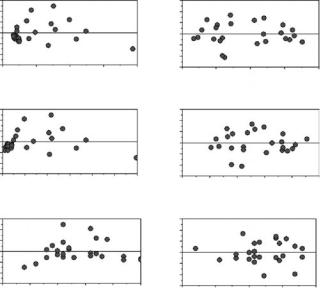
The standardized residuals are plotted on the left-hand side of Figure 3.5 for the regression equation (3.25). There is some suggestion that (a) the variation in the residuals increases with the fitted value or, at any rate, is relatively low for the smallest fitted values, (b) all the residuals are less than zero for lakes with very low phosphorus concentrations, and (c) the residuals are low, then tend to be high, and then tend to be low again as the nitrogen concentration increases.
Std. Residual Std. Residual Std. Residual
3 |
|
|
|
|
|
|
1 |
|
|
|
|
|
|
–1 |
|
|
|
|
|
|
–3 0 |
50 |
100 |
150 |
200 |
||
|
|
Fitted Value |
|
|
||
3 |
|
|
|
|
|
|
1 |
|
|
|
|
|
|
–1 |
|
|
|
|
|
|
–3 0 |
100 |
200 |
300 |
400 |
500 600 |
|
|
|
Phosphorus |
|
|
||
3 |
|
|
|
|
|
|
1 |
|
|
|
|
|
|
–1 |
|
|
|
|
|
|
–3 0 |
5 |
10 |
15 |
20 |
25 |
|
|
|
Nitrogen |
|
|
||
(a)
Std. Residual Std. Residual Std. Residual
3 |
|
|
|
|
1 |
|
|
|
|
–1 |
|
|
|
|
–3 |
1.0 |
1.5 |
2.0 |
2.5 |
0.5 |
Fitted Value
3
1
–1
–30.5 1.0 1.5 2.0 2.5 3.0 Log(Phosphorus)
3
1
–1
–3 0.50 0.75 1.00 1.25 1.50
Log(Nitrogen)
(b)
Figure 3.5
(a) Standardized residuals for chlorophyll-a plotted against the fitted value predicted from the regression equation (3.25) and against the phosphorus and nitrogen concentrations for lakes, and (b) standardized residuals for log(chlorophyll-a) plotted against the fitted value, log(phosphorus), and log(nitrogen) for the regression equation (3.27).

74 Statistics for Environmental Science and Management, Second Edition
Table 3.4
Analysis of Variance for Equation (3.27) Showing the Sums of Squares Accounted for by log(PH) and log(NT) Added into the Equation after log(PH)
|
Sum of |
Degrees of |
Mean |
|
|
Source |
Squares |
Freedom (df) |
Square F-Ratio p-Value |
||
|
|
|
|
|
|
Phosphorus |
5.924 |
1 |
5.924 |
150.98 |
0.0000 |
Nitrogen |
0.303 |
1 |
0.303 |
7.72 |
0.0110 |
Error |
0.863 |
22 |
0.039 |
|
|
|
|
|
|
|
|
Total |
7.090 |
24 |
0.295 |
|
|
|
|
|
|
|
|
The problem here seems to be the particular form assumed for the relationship between chlorophyll-a and the other two variables. It is more usual to assume a linear relationship in terms of logarithms, i.e.,
log(CH) = β0 + β1 log(PH) + β2 log(NT) + ε |
(3.26) |
for the variables being considered (Dominici et al. 1997). Using logarithms to base 10, fitting this equation by multiple regression gives
log(CH) = −1.860 + 1.238 log(PH) + 0.907 log(NT) |
(3.27) |
The R2 value from equation (3.21) is 0.878, which is substantially higher than the value of 0.774 found from fitting equation (3.25). The estimated standard errors for the estimated coefficients of log(PH) and log(NT) are 0.124 and 0.326, respectively, which means that there is strong evidence that log(CH) is related to both of these variables (t = 1.238/0.124 = 9.99 for log(CH), giving p = 0.000 for the t-test with 22 df; t = 0.970/0.326 = 2.78 for log(NT), giving p = 0.011 for the t-test). Finally, the plots of standardized residuals for equation (3.27) that are shown on the right-hand side of Figure 3.5 give little cause for concern.
An analysis of variance is provided for equation (3.27) in Table 3.4. This shows that the equation with log(PH) included accounts for a very highly significant part of the variation in log(CH). Adding in log(NT) to the equation then gives a highly significant improvement.
Insummary,asimplelinearregressionofchlorophyll-aagainstphospho- rus and nitrogen does not seem to fit the data altogether properly, although it accounts for about 77% of the variation in chlorophyll-a. However, by taking logarithms of all the variables, a fit with better properties is obtained, which accounts for about 88% of the variation in log(chlorophyll-a).
3.5 Factorial Analysis of Variance
The analysis of variance that can be carried out with linear regression is very often used in other situations as well, particularly with what are called factorial experiments. An important distinction in this connection is
Models for Data |
75 |
between variables and factors. A variable is something like the phosphorus concentration or nitrogen concentration in lakes, as in the example just considered. A factor, on the other hand, has a number of levels and, in terms of a regression model, it may be thought plausible that the response variable being considered has a mean level that changes with these levels.
Thus if an experiment is carried out to assess the effect of a toxic chemical on the survival time of fish, then the survival time might be related by a regression model to the dose of the chemical, perhaps at four concentrations, which would then be treated as a variable. If the experiment were carried out on fish from three sources, or on three different species of fish, then the type of fish would be a factor, which could not just be entered as a variable. The fish types would be labeled 1 to 3, and what would be required in the regression equation is that the mean survival time varied with the type of fish.
The type of regression model that could then be considered would be
Y = β1X1 + β2X2 + β3X3 + β4X4 + ε |
(3.28) |
where Y is the survival time of a fish; Xi for i = 1 to 3 are dummy indicator variables such that Xi = 1 if the fish is of type i, or is otherwise 0; and X4 is the concentration of the chemical. The effect of this formulation is that, for a fish of type 1, the expected survival time with a concentration of X4 is β1 + β4X4, for a fish of type 2 the expected survival time with this concentration is β2 + β4X4, and for a fish of type 3 the expected survival time with this concentration is β3 + β4X4. Hence, in this situation, the fish type factor at three levels can be allowed for by introducing three 0–1 variables into the regression equation and omitting the constant term β0.
Equation (3.28) allows for a factor effect, but only on the expected survival time. If the effect of the concentration of the toxic chemical may also vary with the type of fish, then the model can be extended to allow for this by adding products of the 0–1 variables for the fish type with the concentration variable to give
Y = β1X1 + β2X2 + β3X3 + β4X1X4 + β5X2X4 + β6X3X4 + ε |
(3.29) |
For fish of types 1 to 3, the expected survival times are then β1 + β4X4, β2 + β5X4, and β3 + β6X4, respectively. The effect is then a linear relationship between the survival time and the concentration of the chemical, which differs for the three types of fish.
When there is only one factor to be considered in a model, it can be handled reasonably easily by using dummy indicator variables as just described. However, with more than one factor, this gets cumbersome, and it is more usual to approach modeling from the point of view of a factorial analysis of variance. This is based on a number of standard models, and the theory can get quite complicated. Nevertheless, the use of analysis of variance in practice can be quite straightforward if a statistical package is available to do the calculations. A detailed introduction to experimental designs and their