

1manly_b_f_j_statistics_for_environmental_science_and_managem
.pdf186 Statistics for Environmental Science and Management, Second Edition
Autocorrelation
1.0
0.8
0.6
0.4
0.2
0.0
–0.2
–0.4
–0.6
0 |
10 |
20 |
30 |
40 |
50 |
Lag (Years)
Figure 8.9
Correlogram for the series of sunspot numbers. The broken horizontal lines indicate the limits on autocorrelations expected for a random series of this length.
8.4 Tests for Randomness
A random time series is one that consists of independent values from the same distribution. There is no serial correlation, and this is the simplest type of data that can occur.
There are a number of standard nonparametric tests for randomness that are sometimes included in statistical packages. These may be useful for a preliminary analysis of a time series to decide whether it is necessary to do a more complicated analysis. They are called “nonparametric” because they are only based on the relative magnitude of observations rather than assuming that these observations come from any particular distribution.
One test is the runs above and below the median test. This involves replacing each value in a series by 1 if it is greater than the median, and 0 if it is less than or equal to the median. The number of runs of the same value is then determined, and compared with the distribution expected if the zeros and ones are in a random order. For example, consider the following series: 1 2 5 4 3 6 7 9 8. The median is 5, so that the series of zeros and ones is 0 0 0 0 0 1 1 1 1. There are M = 2 runs, so this is the test statistic. The trend in the initial series is reflected in M being the smallest possible value. This then needs to be compared with the distribution that is obtained if the zeros and ones are in a random order.
For short series (20 or fewer observations), the observed value of M can be compared with the exact distribution when the null hypothesis is true using tables provided by Swed and Eisenhart (1943), Siegel (1956), or Madansky (1988), among others. For longer series, this distribution is approximately normal with mean
μM = 2r(n − r)]/n + 1 |
(8.6) |
Time Series Analysis |
187 |
and variance |
|
σ2M = 2r(n − r)[2r(n − r) − n]/[n2(n − 1)] |
(8.7) |
where r is the number of zeros (Gibbons 1986, p. 556). Hence |
|
Z = (M − μM)/σM. |
|
can be tested for significance by comparison with the standard normal distribution (possibly modified with the continuity correction described below).
Another nonparametric test is the sign test. In this case the test statistic is P, the number of positive signs for the differences x2 − x1, x3 − x2, …, xn − xn−1. If there are m differences after zeros have been eliminated, then the distribution of P has mean
μP = m/2 |
(8.8) |
and variance |
|
σ2P = m/12 |
(8.9) |
for a random series (Gibbons, 1986, p. 558). The distribution approaches a normal distribution for moderate-length series (say 20 observations or more).
The runs up and down test is also based on the differences between successive terms in the original series. The test statistic is R, the observed number of runs of positive or negative differences. For example, in the case of the series 1 2 5 4 3 6 7 9 8, the signs of the differences are + + − − + + + +, and R = 3. For a random series, the mean and variance of the number of runs are
μR = (2m + 1)/3 |
(8.10) |
and |
|
σ2R = (16m − 13)/90 |
(8.11) |
where m is the number of differences (Gibbons 1986, p. 557). A table of the distribution is provided by Bradley (1968) among others, and C is approximately normally distributed for longer series (20 or more observations).
When using the normal distribution to determine significance levels for these tests of randomness, it is desirable to make a continuity correction to allow for the fact that the test statistics are integers. For example, suppose that there are M runs above and below the median, which is less than the expected number μM. Then the probability of a value this far from μM is twice the integral of the approximating normal distribution from minus infinity to M + ½, provided that M + ½ is less than μM. The reason for taking the integral up to M + ½ rather than M is to take into account the probability of getting exactly M runs, which is approximated by the area from M − ½ to M + ½ under the normal distribution. In a similar way, if M is greater than μM, then twice the area from M − ½ to infinity is the probability of M being this far from μM, provided that M − ½ is greater than μM. If μM lies within the

188 Statistics for Environmental Science and Management, Second Edition
range from M − ½ to M + ½, then the probability of being this far or further from μM is exactly 1.
Example 8.1: Minimum Temperatures in Uppsala, 1900–1981
To illustrate the tests for randomness just described, consider the data in Table 8.1 for July minimum temperatures in Uppsala, Sweden, for the years 1900 to 1981. This is part of a long series started by Anders Celsius, the professor of astronomy at the University of Uppsala, who started collecting daily measurements in the early part of the 18th century. There are almost complete daily temperatures from the year 1739, although true daily minimums are only recorded from 1839, when a maximum– minimum thermometer started to be used (Jandhyala et al. 1999). Minimum temperatures in July are recorded by Jandhyala et al. for the years 1774 to 1981, as read from a figure given by Leadbetter et al. (1983), but for the purpose of this example only the last part of the series is tested for randomness.
A plot of the series is shown in Figure 8.10. The temperatures were low in the early part of the century, but then increased and became fairly constant.
The number of runs above and below the median is M = 42. From equations (8.6) and (8.7), the expected number of runs for a random series is also μM = 32.0, with standard deviation σM = 4.50. Clearly, this is not a significant result. For the sign test, the number of positive differ-
Table 8.1
Minimum July Temperatures in Uppsala (°C), 1900–1981
Year |
Temp |
Year |
Temp |
Year |
Temp |
Year |
Temp |
Year |
Temp |
|
|
|
|
|
|
|
|
|
|
1900 |
5.5 |
1920 |
8.4 |
1940 |
11.0 |
1960 |
9.0 |
1980 |
9.0 |
1901 |
6.7 |
1921 |
9.7 |
1941 |
7.7 |
1961 |
9.9 |
1981 |
12.1 |
1902 |
4.0 |
1922 |
6.9 |
1942 |
9.2 |
1962 |
9.0 |
|
|
1903 |
7.9 |
1923 |
6.7 |
1943 |
6.6 |
1963 |
8.6 |
|
|
1904 |
6.3 |
1924 |
8.0 |
1944 |
7.1 |
1964 |
7.0 |
|
|
1905 |
9.0 |
1925 |
10.0 |
1945 |
8.2 |
1965 |
6.9 |
|
|
1906 |
6.2 |
1926 |
11.0 |
1946 |
10.4 |
1966 |
11.8 |
|
|
1907 |
7.2 |
1927 |
7.9 |
1947 |
10.8 |
1967 |
8.2 |
|
|
1908 |
2.1 |
1928 |
12.9 |
1948 |
10.2 |
1968 |
7.0 |
|
|
1909 |
4.9 |
1929 |
5.5 |
1949 |
9.8 |
1969 |
9.7 |
|
|
1910 |
6.6 |
1930 |
8.3 |
1950 |
7.3 |
1970 |
8.2 |
|
|
1911 |
6.3 |
1931 |
9.9 |
1951 |
8.0 |
1971 |
7.6 |
|
|
1912 |
6.5 |
1932 |
10.4 |
1952 |
6.4 |
1972 |
10.5 |
|
|
1913 |
8.7 |
1933 |
8.7 |
1953 |
9.7 |
1973 |
11.3 |
|
|
1914 |
10.2 |
1934 |
9.3 |
1954 |
11.0 |
1974 |
7.4 |
|
|
1915 |
10.8 |
1935 |
6.5 |
1955 |
10.7 |
1975 |
5.7 |
|
|
1916 |
9.7 |
1936 |
8.3 |
1956 |
9.4 |
1976 |
8.6 |
|
|
1917 |
7.7 |
1937 |
11.0 |
1957 |
8.1 |
1977 |
8.8 |
|
|
1918 |
4.4 |
1938 |
11.3 |
1958 |
8.2 |
1978 |
7.9 |
|
|
1919 |
9.0 |
1939 |
9.2 |
1959 |
7.4 |
1979 |
8.1 |
|
|
|
|
|
|
|
|
|
|
|
|
Time Series Analysis |
189 |
Degrees Celcius
14
12
10
8
6
4
2
0
1900 |
1910 |
1920 |
1930 |
1940 |
1950 |
1960 |
1970 |
1980 |
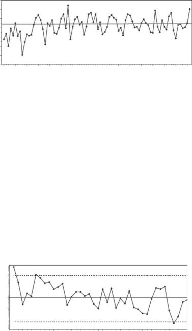
Figure 8.10
Minimum July temperatures in Uppsala, Sweden, for the years 1900 to 1981. The horizontal line shows the mean temperature for the whole period.
ences is P = 44, out of m = 81 nonzero differences. From equations (8.8) and (8.9), the mean and standard deviation for P for a random series are μP = 40.5 and σP = 2.6. With the continuity correction described above, the significance can be determined by comparing Z = (P − ½ − μP)/σP = 1.15 with the standard normal distribution. The probability of a value this far from zero is 0.25. Hence this gives little evidence of nonrandomness. Finally, the observed number of runs up and down is R = 49. From equations (8.10) and (8.11), the mean and standard deviation of R for a random series are μR = 54.3 and σR = 3.8. With the continuity correction, the observed R corresponds to a score of Z = −1.28 for comparing with the standard normal distribution. The probability of a value this far from zero is 0.20, so this is another insignificant result.
None of the nonparametric tests for randomness give any evidence against this hypothesis, even though it appears that the mean of the series was lower in the early part of the century than it has been more recently. This suggests that it is also worth looking at the correlogram, which indicates some correlation in the series from one year to the next. But even here, the evidence for nonrandomness is not very marked (Figure 8.11). The question of whether the mean was constant for this series is considered again in the next section.
Autocorrelation
0.3
0.2
0.1
0.0
–0.1
–0.2
0 |
10 |
20 |
30 |
40 |
|
|
Lag (Years) |
|
|
Figure 8.11
Correlogram for the minimum July temperatures in Uppsala. The 95% limits on autocorrelations for a random series are shown by the broken horizontal lines.

190 Statistics for Environmental Science and Management, Second Edition
8.5 Detection of Change Points and Trends
Suppose that a variable is observed at a number of points of time, to give a time series x1, x2, …, xn. The change-point problem is then to detect a change in the mean of the series if this has occurred at an unknown time between two of the observations. The problem is much easier if the point where a change might have occurred is known, which then requires what is sometimes called an intervention analysis.
A formal test for the existence of a change point seems to have first been proposed by Page (1955) in the context of industrial process control. Since that time, a number of other approaches have been developed, as reviewed by Jandhyala and MacNeill (1986) and Jandhyala et al. (1999). Methods for detecting a change in the mean of an industrial process through control charts and related techniques have been considerably developed (Sections 5.7 and 5.8). Bayesian methods have also been investigated (Carlin et al. 1992), and Sullivan and Woodhall (1996) suggest a useful approach for examining data for a change in the mean or the variance at an unknown time. More recent methods are reviewed by Manly and Chotkowski (2006), who propose two new methods based on bootstrap resampling specifically for data consisting of counts.
The main point to note about the change-point problem is that it is not valid to look at the time series, decide where a change point may have occurred, and then test for a significant difference between the means for the observations before and after the change. This is because the maximum mean difference between two parts of the time series may be quite large by chance alone, and it is liable to be statistically significant if it is tested ignoring the way that it was selected. Some type of allowance for multiple testing (Section 4.9) is therefore needed. See the references given above for details of possible approaches.
A common problem with an environmental time series is the detection of a monotonic trend. Complications include seasonality and serial correlation in the observations. When considering this problem, it is most important to define the time scale that is of interest. As pointed out by Loftis et al. (1991), in most analyses that have been conducted in the past, there has been an implicit assumption that what is of interest is a trend over the time period for which data happen to be available. For example, if 20 yearly results are known, then a 20-year trend has implicitly been of interest. This then means that an increase in the first 10 years followed by a decrease in the last 10 years to the original level has been considered to give no overall trend, with the intermediate changes possibly being thought of as due to serial correlation. This is clearly not appropriate if systematic changes over, say, a five-year period are thought of by managers as being a trend.
When serial correlation is negligible, regression analysis provides a very convenient framework for testing for trends. In simple cases, a regression of the measured variable against time will suffice, with a test to see whether the coefficient of time is significantly different from zero. In more complicated

Time Series Analysis |
191 |
cases, there may be a need to allow for seasonal effects and the influence of one or more exogenous variables. Thus, for example, if the dependent variable is measured monthly, then the type of model that might be investigated is
Yt = β1M1t + β2M2t + … + β12M12t + αXt + θt + εt |
(8.12) |
where Yt is the observation at time t, Mkt is a month indicator that is 1 when the observation is for month k or is otherwise 0, Xt is a relevant covariate measured at time t, and εt is a random error. Then the parameters β1 to β12 allow for differences in Y values related to months of the year, the parameter α allows for an effect of the covariate, and θ is the change in Y per month after adjusting for any seasonal effects and effects due to differences in X from month to month. There is no separate constant term because this is incorporated by the allowance for month effects. If the estimate of θ obtained by fitting the regression equation is significant, then this provides the evidence for a trend.
A small change can be made to the model to test for the existence of seasonal effects. One of the month indicators (say, the first or last) can be omitted from the model and a constant term introduced. A comparison between the fit of the model with just a constant and the model with the constant and month indicators then shows whether the mean value appears to vary from month to month.
If a regression equation such as equation (8.12) is fitted to data, then a check for serial correlation in the error variable εij should always be made. The usual method involves using the Durbin-Watson test (Durbin and Watson 1951), for which the test statistic is
n |
n |
|
V =∑(ei −ei−1)2 |
∑ei2 |
(8.13) |
i=2 |
i=1 |
|
where there are n observations altogether, and e1 to en are the regression residuals in time order. The expected value of V is 2 when there is no autocorrelation. Values less than 2 indicate a tendency for observations that are close in time to be similar (positive autocorrelation), and values greater than 2 indicate a tendency for close observations to be different (negative autocorrelation).
Table A2.5 in Appendix 2 can be used to assess the significance of an observed value of V for a two-sided test at the 5% level. The test is a little unusual, as there are values of V that are definitely not significant, values where the significance is uncertain, and values that are definitely significant. This is explained with the table. The Durbin-Watson test does assume that the regression residuals are normally distributed. It should therefore be used with caution if this does not seem to be the case.
If autocorrelation seems to be present, then the regression model can still be used. However, it should be fitted using a method that is more appropriate
192 Statistics for Environmental Science and Management, Second Edition
than ordinary least-squares. Edwards and Coull (1987), Kutner et al. (2004), and Zetterqvist (1991) all describe how this can be done. Some statistical packages provide one or more of these methods as options. One simple approach is described in Section 8.6 below.
Actually, some researchers have tended to favor nonparametric tests for trend because of the need to analyze large numbers of series with a minimum amount of time devoted to considering the special needs of each series. Thus transformations to normality, choosing models, etc., are to be avoided if possible. The tests for randomness that have been described in the previous section are possibilities in this respect, with all of them being sensitive to trends to some extent. However, the nonparametric methods that currently appear to be most useful are the Mann-Kendall test, the seasonal Kendall test, and the seasonal Kendall test with a correction for serial correlation (Taylor and Loftis 1989; Harcum et al. 1992).
The Mann-Kendall test is appropriate for data that do not display seasonal variation, or for seasonally corrected data, with negligible autocorrelation. For a series x1, x2, …, xn, the test statistic is the sum of the signs of the differences between all pairwise observations,
n |
i-1 |
|
S =∑∑sign(xi −xj ) |
(8.14) |
|
i=2 |
j=1 |
|
where sign(z) is −1 for z < 0, 0 for z = 0, and +1 for z > 0. For a series of values in a random order, the expected value of S is zero and the variance is
Var(S) = n(n − 1)(2n + 5)/18 |
(8.15) |
To test whether S is significantly different from zero, it is best to use a special table if n is 10 or less (Helsel and Hirsch 1992, p. 469). For larger values of n, ZS = S/√Var(S) can be compared with critical values for the standard normal distribution.
To accommodate seasonality in the series being studied, Hirsch et al. (1982) introduced the seasonal Kendall test. This involves calculating the statistic S separately for each of the seasons of the year (weeks, months, etc.) and uses the sum for an overall test. Thus if Sj is the value of S for season j, then on the null hypothesis of no trend, ST = ∑Sj has an expected value of zero and a variance of Var(ST) = ∑Var(Sj). The statistic ZT = ST/√Var(ST) can therefore be used for an overall test of trend by comparing it with the standard normal distribution. Apparently, the normal approximation is good, provided that the total series length is 25 or more.
An assumption with the seasonal Kendall test is that the statistics for the different seasons are independent. When this is not the case, an adjustment for serial correlation can be made when calculating Var(∑ST) (Hirsch and Slack 1984; Zetterqvist 1991). An allowance for missing data can also be made in this case.

Time Series Analysis |
193 |
Finally, an alternative approach for estimating the trend in a series without assuming that it can be approximated by a particular parametric function involves using a moving-average type of approach. Computer packages often offer this type of approach as an option, and more details can be found in specialist texts on time series analysis (e.g., Chatfield 2003).
Example 8.2: Minimum Temperatures in Uppsala, Reconsidered
In Example 8.1, tests for randomness were applied to the data in Table 8.1 on minimum July temperatures in Uppsala for the years 1900 to 1981. None of the tests gave evidence for nonrandomness, although some suggestion of autocorrelation was found. The nonsignificant results seem strange because the plot of the series (Figure 8.10) gives an indication that the minimum temperatures tended to be low in the early part of the century. In this example, the series is therefore reexamined, with evidence for changes in the mean level of the series being specifically considered.
First, consider a regression model for the series, of the form
Yt = β0 + β1t + β2t2 + … + βptp + εt |
(8.16) |
where Yt is the minimum July temperature in year t, taking t = 1 for 1900 and t = 82 for 1981; and εt is a random deviation from the value given by the polynomial for the year t. Trying linear, quadratic, cubic, and quartic models gives the analysis of variance shown in Table 8.2. It is found that the linear and quadratic terms are highly significant, the cubic term is not significant at the 5% level, and the quartic term is not significant at all. A quadratic model therefore seems appropriate.
When a simple regression model like this is fitted to a time series, it is most important to check that the estimated residuals do not display autocorrelation. The Durbin-Watson statistic of equation (8.13) is V = 1.69 for this example. With n = 82 observations and p = 2 regression variables, Table A2.5 shows that, to be definitely significant at the 5% level on a two-sided test, V would have to be less than about 1.52. Hence there is little concern about autocorrelation for this example.
Table 8.2
Analysis of Variance for Polynomial Trend Models Fitted
to the Time Series of Minimum July Temperatures in Uppsala
Source of |
Sum of |
Degrees of |
Mean |
|
Significance |
Variation |
Squares |
Freedom |
Square |
F-ratio |
(p-value) |
|
|
|
|
|
|
Time |
31.64 |
1 |
31.64 |
10.14 |
0.002 |
Time2 |
29.04 |
1 |
29.04 |
9.31 |
0.003 |
Time3 |
9.49 |
1 |
9.49 |
3.04 |
0.085 |
Time4 |
2.23 |
1 |
2.23 |
0.71 |
0.400 |
Error |
240.11 |
77 |
3.12 |
|
|
|
|
|
|
|
|
Total |
312.51 |
81 |
|
|
|
Note: The first four rows of the table show the extra sums of squares accounted for as the linear, quadratic, cubic, and quartic terms added to the model.
194 Statistics for Environmental Science and Management, Second Edition
Standardized Residuals Degrees Celcius
12 |
|
|
|
|
|
|
|
|
8 |
|
|
|
|
|
|
|
|
4 |
|
|
|
|
|
|
|
|
0 1900 |
1910 |
1920 |
1930 |
1940 |
1950 |
1960 |
1970 |
1980 |
3 |
|
|
|
|
|
|
|
|
1 |
|
|
|
|
|
|
|
|
–1 |
|
|
|
|
|
|
|
|
–3 |
1910 |
1920 |
1930 |
1940 |
1950 |
1960 |
1970 |
1980 |
1900 |
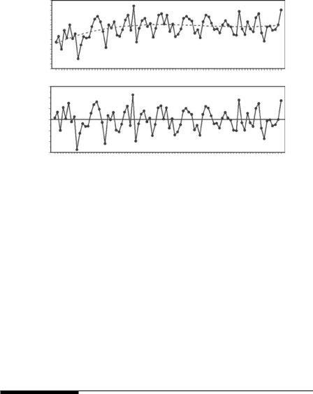
Figure 8.12
A quadratic trend (---) fitted to the series of minimum July temperatures in Uppsala (top graph), with the standardized residuals from the fitted trend (lower graph).
Figure 8.12 shows plots of the original series, the fitted quadratic trend curve, and the standardized residuals (the differences between the observed temperature and the fitted trend values divided by the estimated residual standard deviation). The model appears to be a very satisfactory description of the data, with the expected temperature appearing to increase from 1900 to 1930 and then remain constant, or even decline slightly. The residuals from the regression model are approximately normally distributed, with almost all of the standardized residuals in the range from −2 to +2.
The Mann-Kendall test using the statistic S calculated using equation (8.14) also gives strong evidence of a trend in the mean of this series. The observed value of S is 624, with a standard deviation of 249.7. The Z-score for testing significance is therefore Z = 624/249.7 = 2.50, and the probability of a value this far from zero is 0.012 for a random series.
8.6 More-Complicated Time Series Models
The internal structure of time series can mean that quite complicated models are needed to describe the data. No attempt will be made here to cover the huge amount of literature on this topic. Instead, the most commonly used types of models will be described, with some simple examples of their use. For more information, a specialist text such as that of Chatfield (2003) should be consulted.
The possibility of allowing for autocorrelation with a regression model was mentioned in the last section. Assuming the usual regression situation,
Time Series Analysis |
195 |
where there are n values of a variable Y and corresponding values for variables X1 to Xp, one simple approach that can be used is as follows:
1. Fit the regression model
yt = β0 + β1x1t + … + βp xpt + εt
in the usual way, where yt is the Y value at time t, for which the values of X1 to Xp are x1t to xpt, respectively, and εt is the error term. Let the estimated equation be
yˆ = b0 + b1x1t + … + bp xpt
with estimated regression residuals
et = (yt − yˆt)
2.Assume that the residuals in the original series are correlated because they are related by an equation of the form
εt = αεt−1 + ut
where α is a constant, and ut is a random value from a normal distribution with mean zero and a constant standard deviation. Then it turns out that α can be estimated by αˆ , the first-order serial correlation for the estimated regression residuals.
3. Note that from the original regression model
yt − αyt−1 = β0(1 − α) + β1(x1t − αx1t−1) + … + βp(xpt − αxpt−1) + εt − αεt−1
or
zt = γ + β1v1t + … + βpvpt + ut
where zt = yt − αyt−1, γ = β0(1 − α), and vit = xit − αxit−1, for i = 1, 2, …, p. This is now a regression model with independent errors, so that the
coefficients γ and β1 to βp can be estimated by ordinary regression, with all the usual tests of significance, etc. Of course, α is not known. The approximate procedure actually used is therefore to replace α with the estimate αˆ for the calculation of the zt and vit values.
These calculations can be done easily enough in most statistical packages. A variation called the Cochran-Orcutt procedure involves iterating using steps 2 and 3. What is then done is to recalculate the regression residuals using the estimates of β0 to βp obtained at step 3, obtain a new estimate of α using these, and then repeat step 3. This is continued until the estimate