

1manly_b_f_j_statistics_for_environmental_science_and_managem
.pdf226 |
Statistics for Environmental Science and Management, Second Edition |
|||
|
|
3 |
], h ≤ a |
|
|
γ(h) = c +(S −c)[1.5(h/a)−0.5(h/a) |
|
||
|
c, otherwwise |
|
|
|
|
|
|
|
(9.7) |
|
|
|
|
|
the exponential model with the equation |
|
|
|
|
|
γ(h) = c + (S − c)[1 − exp(−3h/a)] |
(9.8) |
||
and the power model with |
|
|
|
|
|
γ(h) = c + Ahw |
|
|
(9.9) |
For all of these models, c is the nugget effect. The spherical and exponential models also have a sill at S, but for the power model, the function increases without limit as h increases. For the spherical model, the sill is reached when h = a, for the exponential model a is an effective range of influence as γ(a) = c + 0.95(S − c), and for the power model the range of influence is infinite.
A variogram describes the nature of spatial correlation. It may also give information about the correlation between points that are separated by different spatial distances. This is because if Yi and Yj are values of a random variable measured at two locations with the same mean μ, then the expected value of half of the difference squared is
E[0.5(Yi − Yj)2] = 0.5E[(Yi − μ)2 − 2(Yi − μ)(Yj − μ) + (Yj − μ)2]
= 0.5[Var(Yi) − 2Cov(Yi,Yj) + Var(Yj)]
Hence, if the variance is equal to σ2 at both locations, it follows that
E[0.5(Yi − Yj)2] = σ2 − Cov(Yi,Yj)
As the correlation between Yi and Yj is ρ(Yi,Yj) = Cov(Yi,Yj)/σ2, under these conditions, it follows that
E[0.5(Yi − Yj)2] = σ2[1 − ρ(Yi,Yj)]
Suppose also that the correlation between Yi and Yj is only a function of their distance apart, h. This correlation can then be denoted by ρ(h). Finally, note that the left-hand side of the equation is actually the variogram for points distance h apart, so that
γ(h) = σ2[1 − ρ(h)]. |
(9.10) |
This is therefore the function that the variogram is supposed to describe in terms of the variance of the variable being considered and the correlation between points at different distances apart. One important fact that follows
Spatial-Data Analysis |
227 |
is that, because ρ(h) will generally be close to zero for large values of h, the sill of the variogram should equal σ2, the variance of the variable Y being considered.
The requirements for equation (9.10) to hold are that the mean and variance of Y be constant over the study area, and that the correlation between Y at two points depend only on their distance apart. This is called secondorder stationarity. Actually, the requirement for the variogram to exist and to be useful for data analysis is less stringent. This is the so-called intrinsic hypothesis, that the mean of the variable being considered be the same at all locations, with the expected value of 0.5(Yi − Yj)2 depending only on the distance between the locations of the two points (Pannatier 1996, app. A).
Example 9.5: Variograms for SO4 Values of Norwegian Lakes
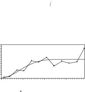
Figure 9.7 shows experimental and model variograms estimated for the SO4 data from Norwegian lakes that are shown in Figure 9.2. The experimental variogram in this case was estimated by taking the maximum distance between two lakes and dividing this into 12 class intervals centered at 0.13, 0.39, 0.73, …, 3.85. The values for 0.5(yi − yj)2 were then averaged within each of these intervals to produce the points that are plotted. For example, for the interval centered at 0.13, covering pairs of points with a distance between them in the range from 0.00 to 0.26, the mean value of 0.5(yi − yj)2 is 0.29. An equation for this variogram is therefore
N(h) |
|
|
|
ˆ |
2 |
N(h) |
(9.11) |
y(h) =∑0.5(yi −yj ) |
|
i=1
where γˆ (h) is the empirical variogram value for the interval centered at a distance h between points, N(h) is the number of pairs of points with a distance between them in this interval, and the summation is over these pairs of points.
|
8 |
|
Variogram |
6 |
|
4 |
||
2 |
||
|
||
|
0 |
0 |
1 |
2 |
3 |
||
|
|
Distance Between Points (h) |
|
||
|
|
Empirical |
|
Gaussian Model |
|
|
|
|
|
||
Figure 9.7
Experimental and model variograms found for the SO4 data on Norwegian lakes displayed in Figure 9.2.

228 Statistics for Environmental Science and Management, Second Edition
The model variogram for Figure 9.7 is the Gaussian model given by equation (9.6). This was estimated using a program produced by the U.S. Environmental Protection Agency called GEOPACK (Yates and Yates 1990) to give
γ(h) = 0.126 + 4.957[1 − exp(−3h2/2.0192)] |
(9.12) |
This is therefore the model function that is plotted in Figure 9.7. The nugget effect is estimated to be 0.126, the sill is estimated to be 0.126 + 4.957 = 5.083, and the range of influence is estimated to be 2.019. Essentially, this model variogram is a smoothed version of the experimental variogram, which is itself a smoothed version of the variogram cloud in Figure 9.5(c). Some standard statistical packages allow function fitting like this and other geostatistical calculations.
9.9 Kriging
Apart from being a device for summarizing the spatial correlation in data, the variogram is also used to characterize this correlation for many other types of geostatistical analyses. There is a great deal that could be said in this respect. However, only one of the commonest of these analyses will be considered here. This is kriging, which is a type of interpolation procedure named after the mining engineer D. G. Krige, who pioneered these methods.
Suppose that, in the study area, sample values y1, y2, …, yn are known at n locations and that it is desired to estimate the value y0 at another location. For simplicity, assume that there are no underlying trends in the values of Y. Then kriging estimates y0 by a linear combination of the known values,
ˆ |
= ∑aiyi |
(9.13) |
y0 |
with the weights a1, a2, …, an for these known values chosen so that the estimator of y0 is unbiased, with the minimum possible variance for prediction errors.
The equations for determining the weights to be used in equation (9.13) are somewhat complicated. They are derived and explained by Thompson (1992, chap. 20) and Goovaerts (1997, chap. 5), among others, and are a function of the assumed model for the variogram. To complicate matters, there are also different types of kriging, with resulting modifications to the basic procedure. For example: Simple kriging assumes that the expected value of the measured variable is constant and known over the entire study region; ordinary kriging allows for the mean to vary in different parts of the study region
Spatial-Data Analysis |
229 |
by only using close observations to estimate an unknown value; and kriging with trend assumes a smooth trend in the mean over the study area.
Ordinary kriging seems to be what is most commonly used. In practice, this is done in three stages:
1.The experimental variogram is calculated to describe the spatial structure in the data.
2.Several variogram models are fitted to the experimental variogram, either by eye or by nonlinear regression methods, and one model is chosen to be the most appropriate.
3.The kriging equations are used to produce estimates of the variable of interest at a number of locations that have not been sampled. Often this is at a grid of points covering the study area.
Example 9.6: Kriging with the SO4 Data
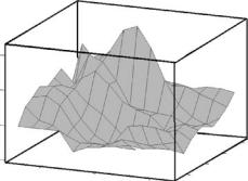
The data on SO4 from Norwegian lakes provided in Figure 9.2 can be used to illustrate the type of results that can be obtained by kriging. A Gaussian variogram for these data is provided by equation (9.12) and displayed graphically in Figure 9.7. This variogram was used to estimate the SO4 level for a grid of points over the study region, with the results obtained being shown in Table 9.3 and Figure 9.8. The calculations were carried out using GEOPACK (Yates and Yates 1990), which produced the estimates and standard errors shown in Table 9.3 using the default values for all parameters. The three-dimensional plot shown in Figure 9.8 was produced using the output saved from GEOPACK.
4 SO
12 |
|
|
|
|
8 |
|
|
|
|
4 |
|
|
|
|
|
|
|
|
12.5 |
0 |
|
|
7.5 |
10.0 |
|
|
titude |
||
58 |
|
5.0 |
||
|
|
|||
60 |
La |
|||
|
62 |
|
|
|
|
Longitude |
|
|
|
|
|
|
|
|
Figure 9.8
Three-dimensional plot of SO4 levels as estimated by applying ordinary kriging to the data shown in Figure 9.2, using the Gaussian variogram shown in Figure 9.7.

230 Statistics for Environmental Science and Management, Second Edition
Table 9.3
Estimated SO4 Values Obtained by Ordinary Kriging Using the Data Shown in the Lower Part of Figure 9.2, with the Standard Errors Associated with These Estimated Values
Latitude |
|
|
|
|
|
Longitude (°East) |
|
|
|
||
|
|
|
|
|
|
|
|
|
|
|
|
(°North) |
4:00 |
5:00 |
6:00 |
7:00 |
8:00 |
9:00 |
10:00 |
11:00 |
12:00 |
13:00 |
|
|
|
|
|
|
|
|
|
||||
Estimation of SO4 Concentrations (mg/l) |
|
|
|
|
|
|
|||||
62:30 |
4.93 |
3.31 |
1.53 |
2.57 |
3.22 |
3.50 |
2.63 |
3.15 |
3.93 |
5.10 |
|
62.00 |
5.29 |
2.93 |
1.80 |
3.56 |
3.78 |
2.82 |
2.48 |
2.23 |
4.57 |
5.37 |
|
61:30 |
5.37 |
2.58 |
1.75 |
3.09 |
3.20 |
2.16 |
2.62 |
2.93 |
5.10 |
5.36 |
|
61:00 |
5.12 |
2.80 |
1.54 |
1.59 |
1.39 |
2.28 |
3.39 |
4.23 |
5.78 |
5.03 |
|
60:30 |
3.14 |
2.95 |
1.76 |
0.79 |
0.52 |
3.76 |
3.51 |
6.80 |
5.68 |
5.36 |
|
60:00 |
2.36 |
1.96 |
1.48 |
0.80 |
0.79 |
4.24 |
3.69 |
10.32 |
6.09 |
5.52 |
|
59:30 |
2.17 |
2.14 |
1.58 |
1.12 |
2.48 |
4.99 |
4.02 |
12.66 |
6.47 |
5.37 |
|
59:00 |
1.50 |
2.03 |
1.57 |
1.95 |
3.89 |
6.75 |
6.70 |
12.03 |
6.22 |
5.58 |
|
58:30 |
3.74 |
2.70 |
3.23 |
3.67 |
4.89 |
8.12 |
8.70 |
9.46 |
6.17 |
6.43 |
|
58:00 |
3.74 |
3.70 |
5.50 |
6.08 |
6.41 |
7.14 |
9.37 |
7.98 |
7.72 |
7.60 |
|
57:30 |
3.74 |
4.13 |
6.46 |
7.03 |
6.66 |
5.57 |
5.77 |
9.97 |
7.60 |
7.60 |
|
57:00 |
3.74 |
5.50 |
6.11 |
6.81 |
6.27 |
6.81 |
7.40 |
3.74 |
3.74 |
3.74 |
|
Standard Errors of Estimates |
|
|
|
|
|
|
|
||||
62:30 |
2.41 |
1.71 |
1.16 |
1.23 |
2.36 |
2.58 |
2.53 |
2.44 |
2.65 |
3.10 |
|
62.00 |
2.07 |
0.81 |
0.55 |
0.51 |
1.90 |
2.21 |
1.99 |
1.70 |
2.29 |
2.80 |
|
61:30 |
1.93 |
0.43 |
0.58 |
0.63 |
1.68 |
1.71 |
1.15 |
0.78 |
1.55 |
2.46 |
|
61:00 |
2.01 |
0.00 |
0.83 |
0.46 |
1.35 |
1.35 |
0.48 |
0.64 |
0.64 |
2.08 |
|
60:30 |
2.45 |
1.01 |
1.04 |
0.73 |
1.01 |
1.11 |
0.53 |
1.03 |
0.49 |
1.81 |
|
60:00 |
2.51 |
1.59 |
0.72 |
0.73 |
0.62 |
0.62 |
0.68 |
0.96 |
0.51 |
2.00 |
|
59:30 |
2.67 |
1.80 |
0.44 |
0.54 |
0.53 |
0.49 |
0.61 |
0.68 |
0.71 |
2.22 |
|
59:00 |
3.10 |
2.02 |
0.51 |
0.48 |
0.51 |
0.47 |
0.85 |
1.10 |
0.70 |
2.36 |
|
58:30 |
2.32 |
2.29 |
0.64 |
0.48 |
0.45 |
0.55 |
1.53 |
1.93 |
1.52 |
2.63 |
|
58:00 |
2.32 |
2.44 |
0.81 |
0.47 |
0.75 |
1.35 |
2.16 |
2.40 |
2.49 |
2.96 |
|
57:30 |
2.32 |
2.73 |
1.50 |
1.21 |
1.59 |
2.11 |
2.67 |
2.96 |
2.95 |
3.10 |
|
57:00 |
2.32 |
3.00 |
2.38 |
2.11 |
2.33 |
2.67 |
3.09 |
2.32 |
2.32 |
2.32 |
|
|
|
|
|
|
|
|
|
|
|
|
|
9.10 Correlation between Variables in Space
When two variables Z1 and Z2 are measured over space at the same n locations and each of the variables displays spatial autocorrelation, then this complicates the problem of deciding whether the two variables are correlated. Certainly it is not valid to calculate the correlation using the set of paired data values and treat this as if it were a random sample of independent pairs of observations for the purpose of deciding whether or not the correlation is statistically significant. Instead, some allowance must be made for the effects of the autocorrelation in the individual variables.

Spatial-Data Analysis |
231 |
In the past, one approach that has been used for handling this problem has used an extension of the Mantel (1967) randomization test as described above. This approach involves calculating three distance matrices. The first is an n × n matrix A in which the element aij in row i and column j is some measure of the difference between the values for Z1 at locations i and j. The second matrix B is of the same size, but the element bij in row i and column j is some measure of the difference between the values of Z2 at locations i and j. Finally, the third matrix G is also of the same size, with the element gij in row i and column j being the geographical distance between locations i and j. The equation
aij = β0 + β1bij + β2gij
is then fitted to the distances by multiple regression, and the significance of the coefficient β1 is tested by comparison with the distribution for this coefficient that is obtained when the labels of the n locations are randomly permuted for the matrix A.
Unfortunately, the general validity of this procedure has proved to be questionable, although it is possible that it can be applied under certain conditions if the n locations are divided into blocks and a form of restricted randomization is carried out (Manly 2007, sec. 9.6). It seems fair to say that this type of approach is still promising, but more work is required to better understand how to overcome problems with its use.
An alternative approach is based on geostatistical methods (Liebhold and Sharov 1997). This involves comparing the observed correlation between two variables, with the distribution obtained from simulated sets of data that are generated in such a way that the variogram for each of the two variables matches the one estimated from the real data, but with the two variables distributed independently of each other. The generation of the values at each location is carried out using a technique called sequential unconditional Gaussian simulation (Borgman et al. 1984; Deutsch and Journel 1992). This method for testing observed correlations is very computer intensive, but it is a reasonable solution to the problem.
9.11 Chapter Summary
•The types of data considered in the chapter are quadrat counts, situations where the location of objects is mapped, and situations where a variable is measured at a number of locations in a study area.
•With quadrat counts, the distribution of the counts will follow a Poisson distribution if objects are randomly located over the study area, independently of each other. The ratio of the variance to the mean (R) is exactly 1 for a Poisson distribution, and this ratio is often
232 Statistics for Environmental Science and Management, Second Edition
used as a measure of clustering, with R > 1 indicating clustering and R < 1 indicating regularity in the location of individuals. A t-test is available to decide whether R is significantly different from 1.
•The Mantel matrix randomization test can be used to see whether quadrats that are close together tend to have different counts. Other randomization tests for spatial correlation are available with the SADIE (Spatial Analysis by Distance IndicEs) computer programs.
•Testing whether two sets of quadrat counts (e.g., individuals of two species counted in the same quadrats) are associated is not straightforward. A randomization test approach involving the production of randomized sets of data with similar spatial structure to the true data appears to be the best approach. One such test is described that is part of the SADIE programs.
•Randomness of point patterns (i.e., whether the points seem to be randomly located in the study area) can be based on comparing the observed mean distances between points and their nearest neighbors with the distributions that are generated by placing the same number of points randomly in the study area using a computer simulation.
•Correlation between two point patterns can also be tested by comparing observed data with computer-generated data. One method involves comparing a statistic that measures the association observed for the real data with the distribution of the same statistic obtained by randomly shifting one of the point patterns. Rotations may be better for this purpose than horizontal and vertical trans lations. The SADIE approach for examining the association between quadrat counts can also be used when the exact locations of points are known.
•A Mantel matrix randomization test can be used to test for spatial autocorrelation using data on a variable measured at a number of locations in a study area.
•A variogram can be used to summarize the nature of the spatial correlation for a variable that can be measured anywhere over a study area, using data from a sample of locations. A variogram cloud is
a plot of 0.5(yi − yj)2 against the distance from point i to point j, for all pairs of sample points, where yi is the value of the variable at the ith sample point. The experimental or empirical variogram is a curve that represents the average observed relationship between
0.5(yi − yj)2 and distance. A model variogram is a mathematical equation fitted to the experimental variogram.
•Kriging is a method for estimating the values of a variable at other than sampled points, using linear combinations of the values at known points. Before kriging is carried out, a variogram model must be fitted using the available data.

Spatial-Data Analysis |
233 |
•In the past, Mantel matrix randomization tests have been used to examine whether two variables measured over space are associated, after allowing for any spatial correlation that might exist for the individual variables. There are potential problems with this application of the Mantel randomization test, which may be overcome by restricting randomizations to points located within spatially defined blocks.
•A geostatistical approach for testing for correlation between two variables X and Y involves comparing the observed correlation between the variables based on data from n sample locations with the distribution of correlations that is obtained from simulated data for which the two variables are independent, but each variable maintains the variogram that is estimated from the real data. Thus the generated correlations are for two variables that individually have spatial correlation structures like those for the real data, although they are actually uncorrelated.
Exercises
Exercise 9.1
Consider the data shown in Figure 2.6 with Example 2.4. These data are concentrations of total PCBs in samples of sediment taken from Liverpool Bay in the United Kingdom. Table 9.4 shows the location of the sampling points and the values for the total PCBs. Use these data to calculate for each pair of locations D1 = geographical distance from one sample to another, D2 = 1/D1, D3 = 0.5(PCB/1000 difference)2, and D4 = 0.5[loge(PCB) difference]2. The purpose of this exercise is to examine the spatial correlation in PCB and loge(PCB) values.
1.Plot D3 and D4 against D1 and D2. Comment on whether serial correlation seems to be present and whether it is more apparent for geographical distances or reciprocal geographical distances. Note that plots of D3 and D4 against D1 are variogram clouds.
2.Use a Mantel randomization test to see whether there is a significant
relationship between D1 and D3, D1 and D4, D2 and D3, and D2 and
D4.
3.Summarize your conclusions about spatial autocorrelation for PCBs in Liverpool Bay.
Exercise 9.2
The geostatistical methods that are discussed in Sections 9.8 and 9.9 typically require the use of special software to do the calculations required. Some of the larger packages have options for doing the calculations, but others do not. There are also some free geostatistical packages available from Web sites, such as the U.S. EPA package GEOPACK. Nevertheless,

234 Statistics for Environmental Science and Management, Second Edition
Table 9.4
Total PCBs in Liverpool Bay Sediments (pg/g)
Station |
X |
Y |
Total PCBs |
Station |
X |
Y |
Total PCBs |
|
|
|
|
|
|
|
|
0 |
29.0 |
19.0 |
1,444 |
34 |
28.7 |
34.5 |
5,990 |
2 |
42.2 |
32.0 |
96 |
35 |
27.0 |
26.0 |
273 |
3 |
42.5 |
34.0 |
1,114 |
36 |
27.0 |
28.5 |
231 |
4 |
42.2 |
37.0 |
4,069 |
37 |
27.0 |
29.7 |
421 |
5 |
39.5 |
30.2 |
266 |
38 |
26.8 |
31.0 |
223 |
6 |
39.7 |
32.5 |
2,599 |
39 |
26.5 |
32.3 |
28,680 |
7 |
40.0 |
35.1 |
2,597 |
40 |
24.8 |
27.3 |
1,084 |
8 |
37.5 |
28.5 |
1,306 |
41 |
24.5 |
29.5 |
401 |
9 |
37.5 |
31.0 |
86 |
42 |
24.5 |
32.0 |
5,702 |
10 |
37.5 |
33.2 |
4,832 |
43 |
24.5 |
34.0 |
2,032 |
11 |
37.5 |
36.0 |
2,890 |
44 |
23.0 |
26.0 |
192 |
12 |
35.5 |
27.3 |
794 |
45 |
22.8 |
27.8 |
321 |
13 |
35.5 |
29.5 |
133 |
46 |
22.0 |
30.6 |
687 |
14 |
35.5 |
31.0 |
1,516 |
47 |
21.8 |
31.5 |
8,767 |
15 |
35.3 |
32.0 |
6,755 |
48 |
21.8 |
32.9 |
4,136 |
16 |
35.5 |
33.0 |
3,621 |
49 |
20.5 |
26.5 |
82 |
17 |
35.7 |
34.0 |
1,870 |
50 |
20.3 |
27.8 |
305 |
18 |
33.0 |
27.8 |
607 |
51 |
20.0 |
29.0 |
2,278 |
19 |
33.0 |
29.0 |
454 |
52 |
19.7 |
31.3 |
633 |
20 |
33.2 |
30.8 |
305 |
53 |
19.2 |
33.8 |
5,218 |
21 |
33.0 |
31.8 |
303 |
54 |
17.8 |
27.5 |
4,160 |
22 |
32.8 |
33.0 |
5,256 |
55 |
17.8 |
28.7 |
2,204 |
23 |
32.8 |
35.2 |
3,153 |
56 |
17.4 |
30.0 |
143 |
24 |
31.0 |
29.0 |
488 |
57 |
17.0 |
32.5 |
5,314 |
25 |
31.0 |
30.2 |
537 |
58 |
17.0 |
34.0 |
2,068 |
26 |
31.0 |
31.3 |
402 |
59 |
15.3 |
28.5 |
17,688 |
27 |
31.0 |
32.7 |
2,384 |
60 |
14.8 |
31.0 |
967 |
28 |
31.2 |
33.8 |
4,486 |
61 |
14.5 |
35.6 |
3,108 |
29 |
29.0 |
27.5 |
359 |
62 |
12.0 |
28.8 |
13,676 |
30 |
29.0 |
30.0 |
473 |
63 |
14.2 |
29.0 |
37,883 |
31 |
28.8 |
31.2 |
1,980 |
64 |
12.6 |
29.6 |
14,339 |
32 |
28.7 |
32.5 |
315 |
65 |
11.5 |
29.2 |
16,143 |
33 |
28.7 |
33.4 |
3,164 |
66 |
13.5 |
28.4 |
13,882 |
Note: X = minutes west of 3° West and Y = minutes north of 53° North.
it is possible to at least fit variograms in a spreadsheet program like Excel. This is what this exercise is about. Begin by considering the two variables D1 and D4 calculated for Exercise 9.1. An exponential variogram is then given by
γ(h) = c + (S − c)[1 − exp(−3h/a)]
Spatial-Data Analysis |
235 |
where γ(h) is the expected value of D4 and h corresponds to the distance D1. This is equation (9.8) from Section 9.8. There are three unknown parameters: c, the nugget effect; a, the range of influence; and S, the sill. Based on the plots made for Exercise 9.1, it should be possible to guess reasonable values for these three parameters. Use the spreadsheet function minimizer (Solver in Excel) to find least-squares estimates of the parameters, starting with the initial guesses. Note that, apart from columns for D1 and D4 in the spreadsheet, it is necessary to make up two further columns, one for the fitted values of γ(h) corresponding to the D1 values, and another for the squared differences between the D4 values and the fitted values. Also, it is necessary to calculate the least-squares fit criterion, which will be the sum of squared differences for all data points. It is the least-squares fit criterion that needs to be minimized in the spreadsheet.