

1manly_b_f_j_statistics_for_environmental_science_and_managem
.pdf196 Statistics for Environmental Science and Management, Second Edition
of α becomes constant to a few decimal places. Another variation that is available in some computer packages is to estimate α and β0 to β1 simultaneously using maximum likelihood.
The validity of this type of approach depends on the simple model εt = αεt−1 + ut being reasonable to account for the autocorrelation in the regression errors. This can be assessed by looking at the correlogram for the series of residuals e1, e2, …, en calculated at step 1 of the above procedure. If the autocorrelations appear to decrease quickly to approximately zero with increasing lags, then the assumption is probably reasonable. This is the case, for example, with the correlogram for Southern Hemisphere temperatures, but is less obviously true for Northern Hemisphere temperatures.
The model εt = αεt−1 + ut is the simplest type of autoregressive model. In general these models take the form
xt = μ + α1(xt−1 − μ) + α2(xt−2 − μ) + … + αp(xt−p − μ) + εt |
(8.17) |
where μ is the mean of the series, α1 to αp are constants, and εt is an error term with a constant variance that is independent of the other terms in the model. This type of model, which is sometimes called AR(p), may be reasonable for series where the value at time t depends only on the previous values of the series plus random disturbances that are accounted for by the error terms. Restrictions are required on the α values to ensure that the series is stationary, which means, in practice, that the mean, variance, and autocorrelations in the series are constant with time.
To determine the number of terms that are required in an autoregressive model, the partial autocorrelation function (PACF) is useful. The pth partial autocorrelation shows how much of the correlation in a series is accounted for by the term αp(xt−p − μ) in the model of equation (8.17), and its estimate is just the estimate of the coefficient αp.
Moving-average models are also commonly used. A time series is said to be a moving-average process of order q, MA(q), if it can be described by an equation of the form
xt = μ + β0zt + β1zt−1 + … + βqzt−q |
(8.18) |
where the values of z1, z2, …, zt are random values from a distribution with mean zero and constant variance. Such models are useful when the autocorrelation in a series drops to close to zero for lags of more than q.
Mixed autoregressive-moving average (ARMA) models combine the features of equations (8.17) and (8.18). Thus an ARMA(p,q) model takes the form
xt = μ + α1(xt−1 − μ) + … + αp(xt−p − μ) + β1zt−1 + … + βqzt−q |
(8.19) |
with the terms defined as before. A further generalization is to integrated autoregressive moving-average models (ARIMA), where differences of the original series are taken before the ARMA model is assumed. The usual

Time Series Analysis |
197 |
reason for this is to remove a trend in the series. Taking differences once removes a linear trend, taking differences twice removes a quadratic trend, and so on. Special methods for accounting for seasonal effects are also available with these models.
Fitting these relatively complicated time series to data is not difficult, as many statistical packages include an ARIMA option, which can be used either with this very general model, or with the component parts such as auto regression. Using and interpreting the results correctly is another matter, and with important time series, it is probably best to get the advice of an expert.
Example 8.3: Temperatures of a Dunedin Stream, 1989 to 1997
For an example of allowing for autocorrelation with a regression model, consider again the monthly temperature readings for a stream in Dunedin, New Zealand. These are plotted in Figure 8.2, and also provided in Table 8.3.
The model that will be assumed for these data is similar to that given by equation (8.12), except that there is a polynomial trend, and no exogenous variable. Thus
Yt = β1M1t + β2M2t + … + β12M12t + θ1t + θ2t2 + … + θptp + εt |
(8.20) |
where Yt is the observation at time t measured in months from 1 in January 1989 to 108 for December 1997; Mkt is a month indicator that is 1 when the observation is in month k, where k goes from 1 for January to 12 for December; and εt is a random error term.
This model was fitted to the data by maximum likelihood using a standard statistical package, assuming the existence of first-order autocorrelation in the error terms so that
εt = αεt−1 + ut. |
(8.21) |
Table 8.3
Monthly Temperatures (°C) for a Stream in Dunedin, New Zealand, 1989–1997
Month |
1989 |
1990 |
1991 |
1992 |
1993 |
1994 |
1995 |
1996 |
1997 |
|
|
|
|
|
|
|
|
|
|
Jan |
21.1 |
16.7 |
14.9 |
17.6 |
14.9 |
16.2 |
15.9 |
16.5 |
15.9 |
Feb |
17.9 |
18.0 |
16.3 |
17.2 |
14.6 |
16.2 |
17.0 |
17.8 |
17.1 |
Mar |
15.7 |
16.7 |
14.4 |
16.7 |
16.6 |
16.9 |
18.3 |
16.8 |
16.7 |
Apr |
13.5 |
13.1 |
15.7 |
12.0 |
11.9 |
13.7 |
13.8 |
13.7 |
12.7 |
May |
11.3 |
11.3 |
10.1 |
10.1 |
10.9 |
12.6 |
12.8 |
13.0 |
10.6 |
Jun |
9.0 |
8.9 |
7.9 |
7.7 |
9.5 |
8.7 |
10.1 |
10.0 |
9.7 |
Jul |
8.7 |
8.4 |
7.3 |
7.5 |
8.5 |
7.8 |
7.9 |
7.8 |
8.1 |
Aug |
8.6 |
8.3 |
6.8 |
7.7 |
8.0 |
9.4 |
7.0 |
7.3 |
6.1 |
Sep |
11.0 |
9.2 |
8.6 |
8.0 |
8.2 |
7.8 |
8.1 |
8.2 |
8.0 |
Oct |
11.8 |
9.7 |
8.9 |
9.0 |
10.2 |
10.5 |
9.5 |
9.0 |
10.0 |
Nov |
13.3 |
13.8 |
11.7 |
11.7 |
12.0 |
10.5 |
10.8 |
10.7 |
11.0 |
Dec |
16.0 |
15.4 |
15.2 |
14.8 |
13.0 |
15.2 |
11.5 |
12.0 |
12.5 |
|
|
|
|
|
|
|
|
|
|

198 Statistics for Environmental Science and Management, Second Edition
Table 8.4
Estimated Parameters for the Model of Equation (8.20) Fitted to the Data on Monthly Temperatures of a Dunedin Stream
|
|
Standard |
|
|
Parameter |
Estimate |
Error |
Ratioa |
P-Valueb |
α (Autoregressive) |
0.1910 |
0.1011 |
1.89 |
0.062 |
β1 (January) |
18.4477 |
0.5938 |
31.07 |
0.000 |
β2 (February) |
18.7556 |
0.5980 |
31.37 |
0.000 |
β3 (March) |
18.4206 |
0.6030 |
30.55 |
0.000 |
β4 (April) |
15.2611 |
0.6081 |
25.10 |
0.000 |
β5 (May) |
13.3561 |
0.6131 |
21.78 |
0.000 |
β6 (June) |
11.0282 |
0.6180 |
17.84 |
0.000 |
β7 (July) |
10.0000 |
0.6229 |
16.05 |
0.000 |
β8 (August) |
9.7157 |
0.6276 |
15.48 |
0.000 |
β9 (September) |
10.6204 |
0.6322 |
16.79 |
0.000 |
β10 (October) |
11.9262 |
0.6367 |
18.73 |
0.000 |
β11 (November) |
13.8394 |
0.6401 |
21.62 |
0.000 |
β12 (December) |
16.1469 |
0.6382 |
25.30 |
0.000 |
θ1 (Time) |
–0.140919 |
0.04117619 |
–3.42 |
0.001 |
θ2 (Time2) |
0.002665 |
0.00087658 |
3.04 |
0.003 |
θ3 (Time3) |
–0.000015 |
0.00000529 |
–2.84 |
0.006 |
aThe estimate divided by the standard error.
bSignificance level for the ratio when compared with the standard normal distribution. The significance levels do not have much meaning for the month parameters, which all have to be greater than zero.
Values of p up to 4 were tried, but there was no significant improvement of the quartic model (p = 4) over the cubic model. Table 8.4 therefore gives the results for the cubic model only. From this table, it will be seen that the estimates of θ1, θ2, and θ3 are all highly significantly different from zero. However, the estimate of the autoregressive parameter is not quite significantly different from zero at the 5% level, suggesting that it may not have been necessary to allow for serial correlation at all. On the other hand, it is safer to allow for serial correlation than to ignore it.
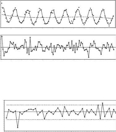
The top graph in Figure 8.13 shows the original data, the expected temperatures according to the fitted model, and the estimated trend. Here the estimated trend is the cubic part of the fitted model, which is −0.140919t + 0.002665t2 − 0.000015t3, with a constant added to make the mean trend value equal to the mean of the original temperature observations. The trend is quite weak, although it is highly significant. The bottom graph shows the estimated ut values from equation (8.21). These should, and do, appear to be random.
There is one further check of the model that is worthwhile. This involves examining the correlogram for the ut series, which should show no significant autocorrelation. The correlogram is shown in Figure 8.14. This is notable for the negative serial correlation of about −0.4 for values
Time Series Analysis |
199 |
Residuals Degrees Celcius
20
15
10
5
0 |
10 |
20 |
30 |
40 |
50 |
60 |
70 |
80 |
90 |
100 |
110 |
3
2
1
0
–1
–2
–3
0 |
10 |
20 |
30 |
40 |
50 |
60 |
70 |
80 |
90 |
100 |
110 |
Month from January 1989
Figure 8.13
The fitted model (—) for the monthly temperature of a Dunedin stream with the estimated trend (---) indicated (top graph), and estimates of the residual components ut in the model (bottom graph).
Autocorrelation
0.2
0.0
–0.2
–0.4
0 |
10 |
20 |
30 |
40 |
50 |
Lag (Months)
Figure 8.14
The correlogram for the estimated random components ut in the model for Dunedin stream temperatures. The 95% limits on autocorrelations for a random series are shown by the broken horizontal lines.
six months apart, which is well outside the limits that should contain 95% of values. There is only one other serial correlation outside these limits, for a lag of 44 months, which is presumably just due to chance. The significant negative serial correlation for a lag of six months indicates that the fitted model is still missing some important aspects of the time series. However, overall the model captures most of the structure, and this curious autocorrelation will not be considered further here.
Example 8.4: Rainfall in Northeast Brazil, 1849–1987
For another example, consider the data shown in Table 8.5 and displayed in Figure 8.15. These are yearly rainfall amounts recorded in rain gauges at Fortaleza in the northeast of Brazil, from 1849 to 1987 (Mitchell 2008). The question to be considered is what is an appropriate model for this series.

200 Statistics for Environmental Science and Management, Second Edition
Table 8.5
Rainfall (cm/year) Measured by Rain Gauges at Fortaleza in Northeast Brazil, 1849–1987
Year |
Rain |
Year |
Rain |
Year |
Rain |
Year |
Rain |
Year |
Rain Year Rain Year Rain |
||||
|
|
|
|
|
|
|
|
|
|
|
|
|
|
1849 |
200.1 |
1869 |
147.0 |
1889 |
78.4 |
1909 |
101.5 |
1929 |
123.0 |
1949 |
188.1 |
1969 |
180.3 |
1850 |
85.2 |
1870 |
162.8 |
1890 |
153.4 |
1910 |
205.1 |
1930 |
110.7 |
1950 |
111.4 |
1970 |
119.2 |
1851 |
180.6 |
1871 |
145.9 |
1891 |
107.7 |
1911 |
137.3 |
1931 |
113.3 |
1951 |
74.7 |
1971 |
209.3 |
1852 |
135.6 |
1872 |
225.6 |
1892 |
121.1 |
1912 |
244.6 |
1932 |
87.9 |
1952 |
137.8 |
1972 |
129.9 |
1853 |
123.3 |
1873 |
205.8 |
1893 |
143.0 |
1913 |
190.5 |
1933 |
93.7 |
1953 |
106.8 |
1973 |
233.1 |
1854 |
159.0 |
1874 |
148.7 |
1894 |
250.5 |
1914 |
151.2 |
1934 |
188.8 |
1954 |
103.2 |
1974 |
251.2 |
1855 |
127.3 |
1875 |
158.1 |
1895 |
249.1 |
1915 |
53.0 |
1935 |
166.1 |
1955 |
115.2 |
1975 |
177.8 |
1856 |
177.0 |
1876 |
156.9 |
1896 |
214.4 |
1916 |
132.8 |
1936 |
82.0 |
1956 |
80.6 |
1976 |
141.7 |
1857 |
173.4 |
1877 |
46.8 |
1897 |
183.9 |
1917 |
207.7 |
1937 |
131.3 |
1957 |
122.5 |
1977 |
194.1 |
1858 |
145.7 |
1878 |
50.3 |
1898 |
86.3 |
1918 |
131.9 |
1938 |
158.6 |
1958 |
50.4 |
1978 |
178.5 |
1859 |
135.7 |
1879 |
59.7 |
1899 |
241.4 |
1919 |
65.6 |
1939 |
191.1 |
1959 |
149.3 |
1979 |
98.5 |
1860 |
171.6 |
1880 |
153.9 |
1900 |
94.0 |
1920 |
184.7 |
1940 |
144.7 |
1960 |
101.1 |
1980 |
109.5 |
1861 |
144.5 |
1881 |
142.3 |
1901 |
154.5 |
1921 |
249.6 |
1941 |
91.6 |
1961 |
175.9 |
1981 |
190.3 |
1862 |
146.8 |
1882 |
124.6 |
1902 |
87.8 |
1922 |
159.5 |
1942 |
78.0 |
1962 |
127.7 |
1982 |
99.9 |
1863 |
145.2 |
1883 |
150.8 |
1903 |
78.9 |
1923 |
151.3 |
1943 |
104.2 |
1963 |
211.0 |
1983 |
81.6 |
1864 |
109.8 |
1884 |
104.7 |
1904 |
113.6 |
1924 |
184.7 |
1944 |
109.0 |
1964 |
242.6 |
1984 |
203.1 |
1865 |
123.8 |
1885 |
130.7 |
1905 |
118.9 |
1925 |
113.7 |
1945 |
175.0 |
1965 |
162.9 |
1985 |
206.6 |
1866 |
247.8 |
1886 |
139.9 |
1906 |
143.0 |
1926 |
157.1 |
1946 |
172.4 |
1966 |
128.9 |
1986 |
214.0 |
1867 |
83.2 |
1887 |
132.0 |
1907 |
69.7 |
1927 |
119.5 |
1947 |
172.6 |
1967 |
193.7 |
1987 |
115.1 |
1868 |
128.9 |
1888 |
73.6 |
1908 |
83.4 |
1928 |
99.5 |
1948 |
138.4 |
1968 |
138.5 |
|
|
|
|
|
|
|
|
|
|
|
|
|
|
|
|
Rainfall (cm/year)
300 |
|
|
|
|
|
|
250 |
|
|
|
|
|
|
200 |
|
|
|
|
|
|
150 |
|
|
|
|
|
|
100 |
|
|
|
|
|
|
50 |
|
|
|
|
|
|
0 |
1880 |
1900 |
1920 |
1940 |
1960 |
1980 |
1860 |
Figure 8.15
Rainfall (cm/year) measured by rain gauges at Fortaleza in northeast Brazil for the years 1849 to 1987. The horizontal line shows the mean rainfall for all years.
The correlogram for the series is shown in Figure 8.16. A first-order autoregressive model and other models including more autoregressive terms and moving-average terms were fitted to the data using the ARIMA option in a standard statistical package, and it was apparent that the first-order autoregressive model is all that is needed. This model was estimated to be
xt = 143.28 + 0.2330(xt−1 − 143.28) + εt |
(8.22) |

Time Series Analysis |
201 |
Autocorrelation
0.3
0.2
0.1
0.0
–0.1
–0.2
0 |
10 |
20 |
30 |
40 |
50 |
60 |
|
|
|
Lag (Years) |
|
|
|
Figure 8.16
Correlogram for the Fortaleza, Brazil, rainfall series, 1849–1987. The 95% limits for the autocorrelations of a random series are shown by the broken horizontal lines.
where the autoregressive coefficient of 0.2330 has an estimated standard error of 0.0832 and is highly significant (t = 2.80, p = 0.005).
The estimated values for the errors εt in the model are approximately normally distributed, with no significant serial correlation. The model of equation (8.22) therefore seems quite satisfactory for these data.
8.7 Frequency Domain Analysis
The analyses considered so far in this chapter are called time domain analyses. They are concerned with modeling the observations directly, with models that are intended to explain the components of an observation xt taken at time t. There is, however, another approach that is used extensively, particularly in areas such as electrical engineering, meteorology, and geophysics. This is called frequency domain analysis, or spectral analysis. Basically, this alternative approach involves attempting to determine how much of the variation in a series is associated with cycles of different lengths. For example, with a 100-year series, it is possible to partition the observed variance into components associated with cycles with lengths of 100 years, 50 years, 33.3 years, 25 years, and so on down to 2 years, the cycle lengths being 100/k, for k equal to 1, 2, …, 50.
This type of analysis has obvious benefits if it cycles in the original series that are of interest. For example, a large part of the variation in the sunspot series (Figure 8.4) is associated with an 11-year cycle. However, many time series analysts find this approach more generally useful for understanding the structure of series.
An introduction to frequency domain analysis of time series is provided by Chatfield (2003). Unfortunately, standard statistical packages often fail to provide any options for doing the required calculations, so specialist software may need to be obtained by those interested in attempting this approach.

202 Statistics for Environmental Science and Management, Second Edition
8.8 Forecasting
There are many reasons for carrying out time series analysis. These include an interest in understanding the structure of the series, deciding whether there is evidence of a significant trend, or deciding whether the mean of the series has changed at some point in time due to some outside influence. Often, however, the analysis is conducted in order to be able to make sensible forecasts of future values of the series, preferably with some idea of the size of the forecasting errors that are likely to occur.
Forecasting of a time series using statistical methods involves extrapolating from the known past and present values into the future. Extrapolation is always dangerous, so anyone who attempts this can expect to be seriously wrong at times. With time series, the problem is that the model may change for some unexpected reason in the future. Or, indeed, the model may be wrong anyway, although it fits the existing data quite well. Actually, models will seldom be exactly correct anyway. Hence, extrapolating an approximate model into the future will probably lead to larger forecasting errors than the model itself suggests. Having said all this, the fact is that it is sometimes very useful to have some idea of what the future values of a time series are likely to be. There is therefore a large amount of literature on this topic.
Some of the methods that are often used, and are available in standard statistical packages, include the following:
1.A trend curve is fitted to the available data and then extrapolated into the future. The trend curve might in this case be linear, a polynomial, or perhaps some more complicated function.
2.Exponential smoothing is used, where the estimate of the mean of a series at time t is the weighted average of past values given by
xˆt = αxt + α(1 − α)xt−1 + α(1 − α)2xt−2 + … + α(1 − α)nxt−n
or equivalently,
xˆt = αxt + (1 − α)xˆt−1 |
(8.23) |
where α is a smoothing constant with a value between 0 and 1. The value of α can be chosen by minimizing the prediction errors for the existing data, and equation (8.23) can then be used to predict into the future, with the actual value of xt replaced by its estimate from the equation. Exponential smoothing can be extended to situations with trend and seasonal variation using something called the HoltWinters procedure (Chatfield 2003).
3.An ARIMA model (Section 8.6) can be fitted to the data and then extrapolated forward. This requires the identification of an appropriate model, which is then predicted forward in time. There are some statistical packages that attempt to do this completely automatically.

Time Series Analysis |
203 |
It would be nice to be able to say which of these methods is generally best. However, this seems impossible because it depends upon the particular circumstances. A detailed discussion of the matters that need to be considered is given by Chatfield (2003).
8.9 Chapter Summary
•Time series analysis may be important because it gives a guide to the underlying process producing a series. It may be necessary to know whether apparent trends and changes in the mean of a series are real, to remove seasonal variation in order to estimate the under lying changes in a series or to forecast the future values of a series.
•The components that often occur in time series are a trend (a tendency to increase or decrease), seasonal variation within the calendar year, other cyclic variation, excursions away from the overall mean for relatively short periods of time, and random variation. These components are displayed in a number of examples that are presented.
•Serial correlation coefficients measure the tendency for observations to be similar or different when they are different distances apart in time. If this tendency exists, then it is also called autocorrelation. A plot of the serial correlation coefficients for different distances apart (lags) is called a correlogram.
•A random time series is one in which each of the observations is an independent random value from the same distribution. There are a number of standard nonparametric tests for randomness. The runs above and below the median, the sign test, and the runs up and down test are described and illustrated on a time series of minimum July temperatures in Uppsala from 1900 to 1981. None of the tests give evidence of nonrandomness.
•The change-point problem involves determining whether there is any evidence of a change in the mean of a time series, without knowing when the change may have occurred. This requires a proper allowance for multiple testing if all possible times of change are considered.
•The detection of trend in an environmental time series is a common problem. In testing for trend, it is important to decide what time scale is important.
•When serial correlation is negligible, regression analysis is a useful tool for detecting trend. A regression model is set up that includes an allowance for trend, and the significance of the estimated trend is tested using the usual regression methods. The Durbin-Watson test can be used to see whether there is serial correlation in the regression

204 Statistics for Environmental Science and Management, Second Edition
residuals. If there is evidence of serial correlation, then the analysis can be modified to allow for this.
•The Mann-Kendall test is a test for monotonic trend in a series when there is no serial correlation. It can be modified to accommodate seasonality in the series being tested, with a correction for serial correlation between seasons if necessary.
•Some more complicated approaches to time series modeling are described: regression models with serially correlated residuals, autoregressive (AR) models, moving average (MA) models, mixed autoregressive-moving average (ARMA) models, and integrated auto regressive moving average (ARIMA) models.
•Frequency domain analysis (spectral analysis) is briefly described.
•Methods for forecasting the future values of a time series (extrapolating a fitted trend, exponential smoothing, and the use of ARIMA models) are briefly described.
Exercises
Exercise 8.1
The data shown in Table 8.6 are pH values read at quarterly intervals for the years 1980 to 1989 for a lake. Carry out the seasonal Mann-Kendall test to see whether there is any evidence of trend in the pH values, and report your conclusions.
Exercise 8.2
Fit a regression model to the data in Table 8.6 to test for trend, using the approach shown in Example 8.2, and report your conclusions. Allow for seasonal effects by treating the four quarters of the year as the four levels
Table 8.6
Quarterly pH Values for a Lake
Year |
Jan–Mar |
Apr–Jun |
Jul–Sep |
Oct–Dec |
|
|
|
|
|
1980 |
5.5 |
7.7 |
6.3 |
4.7 |
1981 |
5.8 |
4.1 |
7.2 |
3.2 |
1982 |
4.6 |
5.2 |
5.2 |
4.4 |
1983 |
7.1 |
6.9 |
5.6 |
6.1 |
1984 |
5.7 |
5.2 |
4.0 |
5.2 |
1985 |
6.6 |
5.5 |
5.3 |
6.3 |
1986 |
6.4 |
6.2 |
5.7 |
8.0 |
1987 |
6.6 |
5.5 |
5.7 |
4.5 |
1988 |
4.5 |
6.1 |
5.2 |
5.0 |
1989 |
6.6 |
4.9 |
7.0 |
6.6 |
|
|
|
|
|

Time Series Analysis |
205 |
Table 8.7
Yearly Wheat Yields (bushels/acre) from Plot 2B at Rothamsted Experimental Station, 1852–1925
Year |
Yield |
Year |
Yield |
Year |
Yield |
Year |
Yield |
|
|
|
|
|
|
|
|
1852 |
1.92 |
1872 |
2.29 |
1892 |
2.37 |
1912 |
1.39 |
1853 |
1.26 |
1873 |
1.82 |
1893 |
2.52 |
1913 |
1.70 |
1854 |
3.00 |
1874 |
2.72 |
1894 |
3.23 |
1914 |
2.26 |
1855 |
2.51 |
1875 |
2.12 |
1895 |
3.17 |
1915 |
2.78 |
1856 |
2.55 |
1876 |
1.73 |
1896 |
3.26 |
1916 |
2.01 |
1857 |
2.90 |
1877 |
1.66 |
1897 |
2.72 |
1917 |
1.23 |
1858 |
2.82 |
1878 |
2.12 |
1898 |
3.03 |
1918 |
2.87 |
1859 |
2.54 |
1879 |
1.19 |
1899 |
3.02 |
1919 |
2.12 |
1860 |
2.09 |
1880 |
2.66 |
1900 |
2.36 |
1920 |
2.39 |
1861 |
2.47 |
1881 |
2.14 |
1901 |
2.83 |
1921 |
2.23 |
1862 |
2.74 |
1882 |
2.25 |
1902 |
2.76 |
1922 |
2.73 |
1863 |
3.23 |
1883 |
2.52 |
1903 |
2.07 |
1923 |
1.51 |
1864 |
2.91 |
1884 |
2.36 |
1904 |
1.63 |
1924 |
1.01 |
1865 |
2.67 |
1885 |
2.82 |
1905 |
3.02 |
1925 |
1.34 |
1866 |
2.32 |
1886 |
2.61 |
1906 |
3.27 |
|
|
1867 |
1.97 |
1887 |
2.51 |
1907 |
2.75 |
|
|
1868 |
2.92 |
1888 |
2.61 |
1908 |
2.97 |
|
|
1869 |
2.53 |
1889 |
2.75 |
1909 |
2.78 |
|
|
1870 |
2.64 |
1890 |
3.49 |
1910 |
2.19 |
|
|
1871 |
2.80 |
1891 |
3.22 |
1911 |
2.84 |
|
|
|
|
|
|
|
|
|
|
of a factor. Once you have decided on an appropriate model for the trend (none, linear, quadratic, etc.), run the Durbin-Watson test to make sure that serial correlation in time does not have to be allowed for.
Exercise 8.3
Table 8.7 shows values for the wheat yield in bushels per acre for Plot 2B of the Broadbank field at Rothamsted Experimental Station, for each of the years 1852 to 1925 (Andrews and Herzberg 1985). During the period covered, this plot was fertilized with farmyard manure only. Carry out analyses on this series similar to the ones shown in Examples 8.1 and 8.2 and report your conclusions concerning any trends, cyclic components, or serial correlation in the series.