

1manly_b_f_j_statistics_for_environmental_science_and_managem
.pdf76 Statistics for Environmental Science and Management, Second Edition
corresponding analyses of variance is presented by Mead et al. (2002). Here, only three simple situations will be considered.
3.5.1 One-Factor Analysis of Variance
With a single factor, the analysis-of-variance model is just a model for comparing the means of I samples, where I is 2 or more. This model can be written as
xij = μ + ai + εij |
(3.30) |
where xij is the jth observed value of the variable of interest at the ith factor level (i.e., in the ith sample), μ is an overall mean level, ai is the deviation from μ for the ith factor level with a1 + a2 + … + aI = 0, and εij is the random component of xij, which is assumed to be independent of all other terms in the model, with a mean of zero and a constant variance.
To test for an effect of the factor, an analysis-of-variance table is set up, which takes the form shown in Table 3.5. Here the sum of squares for the factor is just the sum of squares accounted for by allowing the mean level to change with the factor level in a regression model, although it is usually computed somewhat differently. The F-test requires the assumption that the random components εij in the model of equation (3.30) have a normal distribution.
3.5.2 Two-Factor Analysis of Variance
With a two-factor situation, there are I levels for one factor (A) and J levels for the other factor (B). It is simplest if m observations are taken for each combination of levels, which is what will be assumed here. The model can be written
xijk = μ + ai + bj + (ab)ij + εijk |
(3.31) |
where xijk denotes the kth observation at the ith level for factor A and the jth level for factor B, μ denotes an overall mean level, ai denotes an effect
Table 3.5
Form of the Analysis-of-Variance Table for a One-Factor Model, with I Levels of the Factor and n Observations in Total
Source of |
|
Degrees of |
|
|
Variation |
Sum of Squaresa |
Freedom (df) |
Mean Squareb |
Fc |
Factor |
SSF |
I – 1 |
MSF = SSF/(I – 1) |
MSF/MSE |
Error |
SSE |
n – I |
MSE = SSE/(n – I) |
|
|
|
|
|
|
Total |
SST = ∑∑(xij – x)2 |
n – 1 |
|
|
aSSF = sum of squares between factor levels, SSE = sum of squares for error (variation within factor levels), and SST = total sum of squares for which the summation is over all observations at all factor levels.
bMSF = mean square between factor levels, and MSE = mean square error.
cThe F-value is tested for significance by comparison with critical values for the F-distribution with I − 1 and n − I df.

Models for Data |
77 |
associated with the ith level of factor A, bj denotes an effect associated with the jth level of factor B, (ab)ij denotes an interaction effect so that the mean level at a factor combination does not have to be just the sum of the effects of the two individual factors, and εijk is the random part of the observation xijk, which is assumed to be independent of all other terms in the model, with a mean of zero and a constant variance.
Moving from one to two factors introduces the complication of deciding whether the factors have what are called fixed or random effects, because this can affect the conclusions reached. With a fixed-effects factor, the levels of the factor for which data are collected are regarded as all the levels of interest. The effects associated with that factor are then defined to add to zero. Thus if A has fixed effects, then a1 + a2 + … + aI = 0 and (ab)1j + (ab)2j + … + (ab)Ij = 0, for all j. If, on the contrary, A has random effects, then the values a1 to aI are assumed to be random values from a distribution with mean zero and variance σ2A, while (ab)1j to (ab)Ij are assumed to be random values from a distribution with mean zero and variance σ2AB.
An example of a fixed effect is when an experiment is run with low, medium, and high levels for the amount of a chemical, because in such a case the levels can hardly be thought of as a random choice from a population of possible levels. An example of a random effect is when one of the factors in an experiment is the brood of animals tested, where these broods are randomly chosen from a large population of possible broods. In this case, the brood effects observed in the data will be random values from the distribution of brood effects that are possible.
The distinction between fixed and random effects is important because the way that the significance of factor effects is determined depends on what is assumed about these effects. Some statistical packages allow the user to choose which effects are fixed and which are random, and carries out tests based on this choice. The default is usually fixed effects for all factors, in which case the analysis-of-variance table is as shown in Table 3.6.
Table 3.6
Form of the Analysis-of-Variance Table for a Two-Factor Model with Fixed Effects, and with I Levels for Factor A, J Levels for Factor B, m Observations for Each Combination of Factor Levels, and n = IJm Observations in Total
Source of |
|
|
|
Degrees of |
|
|
Variation |
Sum of Squaresa |
Freedom (df) |
Mean Square |
Fb |
||
Factor A |
SSA |
I – 1 |
MSA = SSA/(I – 1) |
MSA/MSE |
||
Factor B |
SSB |
J – 1 |
MSB = SSB/(J – 1) |
MSB/MSE |
||
Interaction |
SSAB |
(I – 1)(J – 1) |
MSAB = |
MSAB/MSE |
||
|
|
|
|
|
SSAB/[(I – 1)(J – 1)] |
|
Error |
SSE |
IJ(m – 1) |
MSE = SSE/[IJ(m – 1)] |
|
||
|
|
|
|
|
|
|
Total |
SST = ∑∑∑((xijk – |
|
)2 |
n – 1 |
|
|
x |
|
|
||||
aThe sum for SST is over all levels for i, j, and k, i.e., over all n observations.
bThe F-ratios for the factors are for fixed effects only.
78 Statistics for Environmental Science and Management, Second Edition
If there is only m = 1 observation for each factor combination, then the error sum of squares shown in Table 3.6 cannot be calculated. In that case, it is usual to assume that there is no interaction between the two factors, in which case the interaction sum of squares becomes an error sum of squares, and the factor effects are tested using F-ratios that are the factor mean squares divided by this error sum of squares.
3.5.3 Three-Factor Analysis of Variance
With three factors with levels I, J, and K and m observations for each factor combination, the analysis of variance model becomes
xijku = ai + bj + ck + (ab)ij + (ac)ik + (bc)jk + (abc)ijk + εijku |
(3.32) |
where xijku is the uth observation for level i of factor A, level j of factor B, and level k of factor C; ai, bj, and ck are the main effects of the three factors; (ab)ij,
(ac)ik, and (bc)jk are terms that allow for first-order interactions between pairs of factors; (abc)ijk allows for a three-factor interaction (where the mean for a factor combination is not just the sum of the factor and first-order interaction effects); and εijku is a random component of the observation, independent of all other terms in the model, with a mean of zero and a constant variance.
The analysis-of-variance table generalizes in an obvious way in moving from two to three factors. There are now sums of squares, mean squares, and F-ratios for each of the factors, the two-factor interactions, the three-factor interaction, and the error term, as shown in Table 3.7. This table is for all effects fixed. With one or more random effects, some of the F-ratios must be computed differently.
Example 3.2: Survival of Trout in a Metals Mixture
This example concerns part of the results from a series of experiments conducted by Marr et al. (1995) to compare the survival of naive and metals-acclimated juvenile brown trout (Salmo trutta) and rainbow trout (Oncorhynchus mykiss) when exposed to a metals mixture with the maximum concentrations found in the Clark Fork River, Montana.
In the trials, called Challenge 1, there were three groups of fish (hatchery brown trout, hatchery rainbow trout, and Clark Fork River brown trout). Approximately half of each group (randomly selected) were controls that were kept in clean water for three weeks before being transferred to the metals mixture. The other fish in each group were acclimated for three weeks in a weak solution of metals before being transferred to the stronger mixture. All fish survived the initial threeweek period, and an outcome variable of interest was the survival time of the fish in the stronger mixture. The results from the trials are shown in Table 3.8.
The results from this experiment can be analyzed using the two-factor analysis-of-variance model. The first factor is the type of fish, which is

Models for Data |
79 |
Table 3.7
Form of the Analysis-of-Variance Table for a Three-Factor Model with Fixed Effects
Source of |
Sum of |
Degrees of |
|
|
||
Variation |
Squaresa |
Freedom (df) |
Mean Square |
Fb |
||
Factor A |
SSA |
I – 1 |
MSA = SSA/(I – 1) |
MSA/MSE |
||
Factor B |
SSB |
J – 1 |
MSB = SSB/(J – 1) |
MSB/MSE |
||
Factor C |
SSC |
K – 1 |
MSC = SSC/(K – 1) |
MSC/MSE |
||
AB interaction |
SSAB |
(I – 1)(J – 1) |
MSAB = |
MSAB/MSE |
||
|
|
|
|
|
SSAB/[(I – 1)(J – 1)] |
|
AC interaction |
SSAC |
(I – 1)(K – 1) |
MSAC = |
MSAC/MSE |
||
|
|
|
|
|
SSAC/[(I – 1)(K – 1)] |
|
BC interaction |
SSBC |
(J – 1)(K – 1) |
MSBC = |
MSBC/MSE |
||
|
|
|
|
|
SSBC/[(J – 1)(K – 1)] |
|
ABC interaction |
SSABC |
(I – 1)(J – 1) |
MSABC = |
MSABC/MSE |
||
|
|
|
|
(K – 1) |
SSABC/[(I – 1)(J – 1)(K – 1)] |
|
Error |
SSE |
IJK(m – 1) |
MSE = |
|
||
|
|
|
|
|
SSE/[IJK(m – 1)] |
|
|
|
|
|
|
|
|
Total |
SST = |
n – 1 |
|
|
||
|
∑∑∑∑(xijk – |
|
)2 |
|
|
|
|
x |
|
|
|
||
Note: I Levels for factor A, J Levels for factor B, K Levels for factor C, m observations for each combination of factor levels, and n = IJMm observations in total
aThe sum for SST is over all levels for i, j , k, and m, i.e., over all n observations.
bThe F-ratios for the factors and two-factor interactions are for fixed effects only.
at three levels (two types of brown trout and one type of rainbow trout). This is a fixed-effects factor because no other types of fish are being considered. The second factor is the treatment, which is at two levels (control and acclimated). Again, this is a fixed-effects factor because no other treatments are being considered. A slight complication is the unequal numbers of fish at the different factor combinations. However, many statistical packages can allow for this reasonably easily. The analysis presented here was carried out with the general linear model option in MINITAB (Minitab 2008).
A second complication is the increase in the variation in the survival time as the mean increases. It can be seen, for example, that the lowest mean survival time shown in Table 3.8 (21.53 h) is for control hatchery brown trout. This group also has the lowest standard deviation (4.72 h). This can be compared with the highest mean survival time (69.00 h) for acclimated Clark Fork River brown trout, which also has the highest standard deviation (35.25 h). It seems, therefore, that the assumption of a constant variance for the random component in the model presented in equation (3.31) is questionable. This problem can be overcome for this example by analyzing the logarithm of the survival time rather than the survival time itself. This largely removes the apparent relationship between means and variances.
The analysis of variance is shown in Table 3.9 for logarithms to base 10. Starting from a model with no effects, adding the species factor gives

80 Statistics for Environmental Science and Management, Second Edition
Table 3.8
Results from Challenge 1 Experiment, Where the Effect of an Acclimatization Treatment on Survival Was Examined for Three Types of Fish
|
|
|
|
Survival Time (h) |
|
|
|
|
|
Hatchery Brown Trout |
|
Hatchery Rainbow Trout |
|
Clark Fork Brown Trout |
|||
|
Control |
Treated |
|
Control |
Treated |
|
Control |
Treated |
|
|
|
|
|
|
|
|
|
|
8 |
10 |
24 |
54 |
30 |
36 |
||
|
18 |
60 |
24 |
48 |
30 |
30 |
||
|
24 |
60 |
24 |
48 |
30 |
30 |
||
|
24 |
60 |
24 |
54 |
36 |
30 |
||
|
24 |
54 |
24 |
54 |
30 |
36 |
||
|
24 |
72 |
24 |
36 |
36 |
30 |
||
|
18 |
54 |
24 |
30 |
36 |
42 |
||
|
18 |
30 |
24 |
18 |
24 |
54 |
||
|
24 |
36 |
24 |
48 |
36 |
30 |
||
|
18 |
48 |
24 |
36 |
36 |
48 |
||
|
10 |
48 |
24 |
24 |
36 |
24 |
||
|
24 |
42 |
18 |
24 |
30 |
54 |
||
|
24 |
54 |
18 |
48 |
18 |
54 |
||
|
24 |
10 |
24 |
48 |
30 |
36 |
||
|
10 |
66 |
30 |
36 |
24 |
30 |
||
|
18 |
42 |
30 |
42 |
30 |
90 |
||
|
24 |
36 |
30 |
36 |
24 |
60 |
||
|
24 |
42 |
30 |
36 |
30 |
66 |
||
|
24 |
36 |
36 |
42 |
42 |
108 |
||
|
24 |
36 |
30 |
36 |
42 |
114 |
||
|
24 |
36 |
30 |
36 |
24 |
108 |
||
|
24 |
36 |
30 |
36 |
10 |
114 |
||
|
24 |
36 |
30 |
36 |
24 |
120 |
||
|
24 |
36 |
30 |
42 |
24 |
90 |
||
|
24 |
30 |
36 |
42 |
24 |
96 |
||
|
24 |
30 |
36 |
36 |
36 |
30 |
||
|
24 |
36 |
36 |
36 |
24 |
108 |
||
|
24 |
30 |
36 |
36 |
30 |
108 |
||
|
24 |
36 |
36 |
36 |
18 |
108 |
||
|
24 |
36 |
36 |
|
24 |
102 |
||
|
|
|
|
|
|
|
|
102 |
|
|
|
|
|
|
|
|
120 |
|
|
|
|
|
|
|
|
|
n |
30 |
30 |
30 |
29 |
30 |
32 |
||
Mean |
21.53 |
41.27 |
28.20 |
39.10 |
28.93 |
69.00 |
||
Std. Dev. |
4.72 |
14.33 |
|
5.49 |
8.87 |
|
7.23 |
35.25 |
Source: Marr et al. (1995).

Models for Data |
81 |
Table 3.9
Analysis of Variance on Logarithms to Base 10 of the Daily Survival Times Shown in Table 3.8
Source of |
Sum of |
Degrees of |
|
|
|
Variation |
Squaresa |
Freedom (df) |
Mean Square |
F |
p-Value |
Species |
0.863 |
2 |
0.431 |
17.20 |
0.000 |
Treatment |
2.719 |
1 |
2.719 |
108.39 |
0.000 |
Interaction |
0.287 |
2 |
0.143 |
5.72 |
0.004 |
Error |
4.389 |
175 |
0.025 |
|
|
|
|
|
|
|
|
Total |
8.257 |
180 |
|
|
|
aThe sums of squares shown here depend on the order in which effects are added into the model, which is species, then the treatment, and finally the interaction between these two factors.
a very highly significant improvement in the fit of the model (F = 17.20, p = 0.000). Adding the main effect of treatment leads to another very highly significant improvement in fit (F = 108.39, p = 0.000). Finally, adding in the interaction gives a highly significant improvement in the fit of the model (F = 5.72, p = 0.004). It can therefore be concluded that the mean value of the logarithm of the survival time varies with the species and with the acclimation treatment. Also, because of the interaction that seems to be present, the effect of the acclimation treatment is not the same for all three types of fish.
On a logarithmic scale, a treatment has no interaction when the proportional change that it causes is constant. For the Challenge 1 trials, the interaction is significant because the effect of acclimation varies considerably with the three types of fish. For hatchery brown trout, the mean survival time for acclimated fish (41.3 h) was 92% higher than the mean survival time for the controls (21.5 h); for hatchery rainbow trout, the mean survival time for acclimated fish (39.1 h) was 39% higher than the mean survival time for the controls (28.2 h); and for Clark Fork River brown trout the mean survival time for the acclimated fish (69.0 h) was 139% higher than the mean survival time for the controls (28.9 h). The proportional changes are therefore very far from being constant.
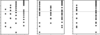
The assumptions of the analysis-of-variance model seem fairly reasonable for this example after the survival times are transformed to logarithms, as can be seen from the plots of standardized residuals that are shown in Figure 3.6. For a good fitting model, most of the standardized residuals should be within the range −2 to +2, which they are. There are, however, some standardized residuals less than −2, and one of nearly −4. There is also a suggestion that the amount of variation is relatively low for fish with a small expected survival time, the second type of fish (hatchery rainbow trout), and treatment 1 (the controls). These effects are not clear enough to cause much concern.
82 Statistics for Environmental Science and Management, Second Edition
Standardized Residual
2 |
|
|
2 |
|
|
2 |
|
0 |
|
|
0 |
|
|
0 |
|
–2 |
|
|
–2 |
|
|
–2 |
|
–4 |
1.6 |
1.8 |
–4 |
2 |
3 |
–4 |
2 |
1.4 |
1 |
1 |
|||||
Fitted Value |
|
|
Type of Fish |
|
|
Treatment |
|
Figure 3.6
Plots of standardized residuals against fitted values, the type of fish, and the treatment from the analysis of variance model for the logarithm of survival times from Marr et al.’s (1995) Challenge 1 trials.
3.5.4 Repeated-Measures Designs
Many environmental data sets have a repeated-measures type of design. An example would be vegetation monitoring to assess the effect of alternative control strategies on browsing pests, such as possums in New Zealand. There might, for example, be three areas: one with no pest control, one with some pest control, and one with intensive pest control. Within each area, four randomly placed plots might be set up, and then the percentage foliage cover measured for six years on those plots. This would then result in data of the form shown in Table 3.10.
In this example, the area is a between-plot factor at three levels, and the year is a within-plot factor. There is a special option in many statistics packages to analyze data of this type, and there can be more than one betweenplot factor, and more than one within-plot factor. A set of data like that shown in Table 3.10 should not be analyzed as a factorial design with three factors (area, year, and plot), because that assumes that the plots in different areas match up, e.g., plot 1 in areas 1, 2, and 3 have something similar about them, which will generally not be true. Rather, the numbering of plots within areas will be arbitrary, which is sometimes referred to as plots being nested within areas. On the other hand, a repeated-measures analysis of variance does assume that the measurements at different times on one plot in one area tend to be similar. Thus it is one way of overcoming the problem of pseudoreplication, which is discussed further in Section 4.8.
An important special application of repeated-measures analysis of variance is with the before–after-control-impact (BACI) and other designs that are discussed in Chapter 6. In this case, there may be a group of sites that are controls, with no potential impact, and another group of sites that are potentially impacted. Repeated observations are made on the sites at different times over the study period, and at some point in time there is an event

Models for Data |
83 |
Table 3.10
The Form of Data from a Repeated-Measures Experiment with Four Plots in Each of Three Different Treatment Areas Measured for Six Years
Area |
Plot |
Year 1 |
Year 2 |
Year 3 |
Year 4 |
Year 5 |
Year 6 |
|
|
|
|
|
|
|
|
No pest control |
1 |
X |
X |
X |
X |
X |
X |
|
2 |
X |
X |
X |
X |
X |
X |
|
3 |
X |
X |
X |
X |
X |
X |
|
4 |
X |
X |
X |
X |
X |
X |
Low pest control |
1 |
X |
X |
X |
X |
X |
X |
|
2 |
X |
X |
X |
X |
X |
X |
|
3 |
X |
X |
X |
X |
X |
X |
|
4 |
X |
X |
X |
X |
X |
X |
High pest control |
1 |
X |
X |
X |
X |
X |
X |
|
2 |
X |
X |
X |
X |
X |
X |
|
3 |
X |
X |
X |
X |
X |
X |
|
4 |
X |
X |
X |
X |
X |
X |
Note: A measurement of percentage foliage cover is indicated by X.
at the sites that may be impacted. The question then is whether the event has a detectable effect on the observations at the impact sites.
The analysis of designs with repeated measures can be quite complicated, and it is important to make the right assumptions (Von Ende 1993). This is one area where expert advice may need to be sought.
3.5.5 Multiple Comparisons and Contrasts
Many statistical packages for analysis of variance allow the user to make comparisons of the mean level of the dependent variable for different factor combinations, with the number of multiple comparisons being allowed for in various ways. Multiple testing methods are discussed further in Section 4.9. Basically, they are a way to ensure that the number of significant results is controlled when a number of tests of significance are carried out at the same time, with all the null hypotheses being true. Or, alternatively, the same methods can be used to ensure that when a number of confidence intervals are calculated at the same time, then they will all contain the true parameter value with a high probability.
There are often many options available with statistical packages, and the help facility with the package should be read carefully before deciding which, if any, of these to use. The use of a Bonferroni correction is one possibility that is straightforward and usually available, although this may not have the power of other methods.
Be warned that some statisticians do not like multiple comparison methods. To quote one leading expert on the design and analysis of experiments (Mead 1988, p. 310):

84 Statistics for Environmental Science and Management, Second Edition
Although each of these methods for multiple comparisons was developed for a particular, usually very limited, situation, in practice these methods are used very widely with no apparent thought as to their appropriateness. For many experimenters, and even editors of journals, they have become automatic in the less desirable sense of being used as a substitute for thought.… I recommend strongly that multiple comparison methods be avoided unless, after some thought and identifying the situation for which the test you are considering was proposed, you decide that the method is exactly appropriate.
He goes on to suggest that simple graphs of means against factor levels will often be much more informative than multiple comparison tests.
On the other hand, Mead (1988) does make use of contrasts for interpreting experimental results, where these are linear combinations of mean values that reflect some aspect of the data that is of particular interest. For example, if observations are available for several years, then one contrast might be the mean value in year 1 compared with the mean value for all other years combined. Alternatively, a set of contrasts might be based on comparing each of the other years with year 1. Statistical packages often offer the possibility of considering either a standard set of contrasts, or contrasts defined by the user.
3.6 Generalized Linear Models
The regression and analysis-of-variance models described in the previous two sections can be considered to be special cases of a general class of generalized linear models. These were first defined by Nelder and Wedderburn (1972), and include many of the regression types of models that are likely to be of most use for analyzing environmental data. A very thorough description of the models and the theory behind them is provided by McCullagh and Nelder (1989).
The characteristic of generalized linear models is that there is a dependent variable Y, which is related to some other variables X1, X2, …, Xp by an equation of the form
Y = f(β0 + β1X1 + β2X2 + … + βpXp) + ε |
(3.33) |
where f(x) is one of a number of allowed functions, and ε is a random value with a mean of zero from one of a number of allowed distributions. For example, setting f(x) = x and assuming a normal distribution for ε just gives the usual multiple regression model of equation (3.17).
Setting f(x) = exp(x) makes the expected value of Y equal to
E(Y) = exp(β0 + β1X1 + β2X2 + … + βpXp) |
(3.34) |
Models for Data |
85 |
Assuming that Y has a Poisson distribution then gives a log-linear model, which is a popular assumption for analyzing count data. The description log-linear comes about because the logarithm of the expected value of Y is a linear combination of the X variables.
Alternatively, setting f(x) = exp(x)/[1 + exp(x)] makes the expected value of Y equal to
E(Y) = exp(β0 + β1X1 + … + βpXp)/[1 + exp(β0 + β1X1 + … + βpXp)] (3.35)
This is the logistic model for a random variable Y that takes the value 0 (indicating the absence of an event) or 1 (indicating that an event occurs), where the probability of Y = 1 is given as a function of the X variables by the righthand side of equation (3.35).
There are many other possibilities for modeling within this framework using many of the standard statistical packages currently available. Table 3.11 gives a summary of the most common models that are used.
Generalized linear models are usually fitted to data using the principle of maximum likelihood, i.e., the unknown parameter values are estimated as those values that make the probability of the observed data as large as possible. This principle is one that is often used in statistics for estimation. Here it is merely noted that the goodness of fit of a model is measured by the deviance, which is (apart from a constant) minus twice the maximized log-likelihood, with associated degrees of freedom equal to the number of observations minus the number of estimated parameters.
With models for count data with Poisson errors, the deviance gives a direct measure of absolute goodness of fit. If the deviance is significantly large in comparison with critical values from the chi-squared distribution, then the model is a poor fit to the data. Conversely, a deviance that is not significantly large shows that the model is a good fit. Similarly, with data consisting of proportions with binomial errors, the deviance is an absolute measure of the goodness of fit when compared with the chi-squared distribution, provided that the numbers of trials that the proportions relate to (n in Table 3.11) are not too small, say, generally more than five.
With data from distributions other than the Poisson or binomial, or for binomial data with small numbers of trials, the deviance can only be used as a relative measure of goodness of fit. The key result then is that—if one model has a deviance of D1 with ν1 df and another model has a deviance of D2 with ν2 df, and the first model contains all of the parameters in the second model plus some others—then the first model gives a significantly better fit than the second model if the difference D2 − D1 is significantly large in comparison with the chi-squared distribution with ν2 − ν1 df. Comparing several models in this way is called an analysis of deviance by analogy to the analysis of variance. These tests using deviances are approximate, but they should give reasonable results, except perhaps with rather small sets of data.