

1manly_b_f_j_statistics_for_environmental_science_and_managem
.pdf46 Statistics for Environmental Science and Management, Second Edition
procedure on all 90 units, a ranked-set sample of size 30 is available based on the accurate estimation of density. This sample is not as good as would have been obtained by measuring all 90 units accurately, but it should have considerably better precision than a standard sample of size 30.
Let m be the size of the ranked set (3 in the above example), so that one cycle of ranking and measurement uses m2 units, accurately measuring first the highest of m units then the second highest of m units, and so on. Also, let k be the number of times that the cycle is repeated (10 in the above example), so that n = km values are accurately measured in total. Then it can be shown that if there are no errors in the ranking of the sets of size m and if the distribution of the variable being measured is unimodal, the ratio of the variance of the mean from ranked-set sampling to the variance of the mean for a simple random sample of size n is slightly more than 2/(m + 1). Thus, in the example with m = 3 and a ranked-set sample size of 30, the variance of the sample mean should be slightly more than 2/(3 + 1) = 1/2 of the variance of a simple random sample of size 30.
In practice, the user of ranked-set sampling has two alternatives in terms of assessing the error in estimating a population mean using the mean of the ranked-set sample. If there are few, if any, errors in ranking, and if the distribution of data values in the population being studied can be assumed to be unimodal, then the standard error of the ranked-set sample mean can be estimated approximately by
SÊ(x) = √{[2/(m + 1)](s2/n)} |
(2.30) |
Alternatively, the sample can conservatively be treated as being equivalent to a simple random sample of size n, in which case the estimated standard error
SÊ(x) = s/√n |
(2.31) |
will almost certainly be too large.
For a further discussion and more details about ranked-set sampling, see the review by Patil et al. (1994) and the special issue of the journal Environmental and Ecological Statistics on this topic (Ross and Stokes 1999). For reviews of the alternative methods that may be applied for environmental sampling, two U.S. Environmental Protection Agency reports are relevant (US EPA 2002a, 2002b).
2.11 Ratio Estimation
Occasions arise where the estimation of the population mean or total for a variable X is assisted by information on a subsidiary variable U. What is required is that the items in a random sample of size n have values x1 to xn
Environmental Sampling |
47 |
for X, and corresponding values u1 to un for U. In addition, μu, the population mean for U, and Tu = Nμu, the population total for U, must be known values. An example of such a situation would be where the level of a chemical was measured some years ago for all of the sample units in a population, and it is required to estimate the current mean level from a simple random sample of the units. Then the level of the chemical from the earlier survey is the variable U, and the current level is the variable X.
With ratio estimation, it is assumed that X and U are approximately proportional, so that X ≈ RU, where R is some constant. The value of the ratio R of X to U can then be estimated from the sample data by
r = x/u |
(2.32) |
and hence the population mean of X can be estimated by multiplying r by the population mean of U, to get
xratio = rμu |
(2.33) |
which is the ratio estimator of the population mean. Multiplying both sides of this equation by the population size N, the ratio estimate of the population total for X is found to be
tX = rTu |
(2.34) |
If the ratio of X to U is relatively constant for the units in a population, then the ratio estimator of the population mean for X can be expected to have lower standard errors than the sample mean x. Similarly, the ratio estimator of the population total for X should have a lower standard error than Nx. This is because the ratio estimators allow for the fact that the observed sample may, by chance alone, consist of items with rather low or high values for X. Even if the random sample does not reflect the population very well, the estimate of r may still be reasonable, which is all that is required for a good estimate of the population total.
The variance of xratio can be estimated by
|
n |
|
|
|
ˆ |
2 |
/[(n −1)n][1 |
−(n/N)] |
(2.35) |
Var(xratio ) ≈∑(xi −rui ) |
||||
i=1
An approximate 100(1 − α)% confidence interval for the population mean of X is then given by
xratio ± zα/2 SÊ(xratio) |
(2.36) |
where SÊ(xratio) = √Vâr(xratio) and, as before, zα/2 is the value from the standard normal distribution that is exceeded with probability α/2.
48 Statistics for Environmental Science and Management, Second Edition
Because the ratio estimator of the population total of X is tx = Nxratio, it also follows that
SÊ(tX) ≈ N SÊ(xratio) |
(2.37) |
and an approximate 100(1 − α)% confidence interval for the true total is given by
tX ± zα/2 SÊ(tx) |
(2.38) |
The equations for variances, standard errors, and confidence intervals should give reasonable results, provided that the sample size n is large (which in practice means 30 or more) and that the coefficients of variation of x and u (the standard errors of these sample means divided by their population means) are less than 0.1 (Cochran 1977, p. 153).
Ratio estimation assumes that the ratio of the variable of interest X to the subsidiary variable U is approximately constant for the items in the population. A less restrictive assumption is that X and U are related by an equation of the form X ≈ α + βU, where α and β are constants. This then allows regression estimation to be used. See Manly (1992, chap. 2) for more information about this generalization of ratio estimation.
Example 2.5: pH Levels in Norwegian Lakes
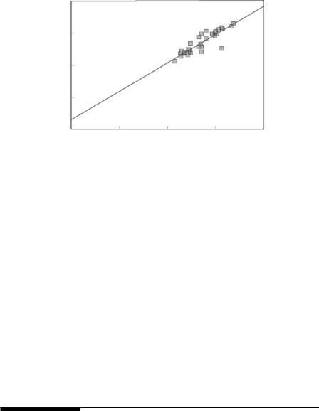
Example 1.2 was concerned with a Norwegian study that was started in 1972 to investigate the effects of acid precipitation. As part of this study, the pH levels of 46 lakes were measured in 1976, and for 32 of the lakes the pH level was measured again in 1977. The results are shown in Table 2.6 for the 32 lakes that were measured in both years. The present example is concerned with the estimation of the mean pH level for the population of 46 lakes in 1977 using the ratio method. Figure 2.8 shows a plot of the 1977 pH values against the 1976 pH values for the 32 lakes. Because a line through the data passes nearly through the origin, there is approximately a ratio relationship, so that ratio estimation is justified.
For ratio estimation, the pH level in a lake in 1976 is the auxiliary variable (U), and the pH level in 1977 is the main variable of interest (X). The mean of U for the 46 lakes is known to be 5.345 in 1976. For the 32 lakes sampled in 1977, the mean of U is u = 5.416, and the mean of X is x = 5.400. Therefore the estimated ratio of X to U is
r = 5.400/5.416 = 0.997
The ratio estimate of the mean pH for all 46 lakes in 1977 is therefore given by equation (2.33) to be
xratio = 0.997 × 5.345 = 5.329
The column headed X − rU in Table 2.6 gives the values required for the summation on the right-hand side of equation (2.35). The sum of this

Environmental Sampling |
49 |
Table 2.6
Values for pH Measured on 32 Norwegian Lakes in 1976 and 1977
|
|
|
pH |
|
|
|
|
1976 |
1977 |
|
|
Lake |
Id |
U |
|
X |
X − rU |
|
|
|
|
|
|
1 |
4 |
4.32 |
4.23 |
−0.077 |
|
2 |
5 |
4.97 |
4.74 |
−0.215 |
|
3 |
6 |
4.58 |
4.55 |
−0.016 |
|
4 |
8 |
4.72 |
4.81 |
0.104 |
|
5 |
9 |
4.53 |
4.70 |
0.184 |
|
6 |
10 |
4.96 |
5.35 |
0.405 |
|
7 |
11 |
5.31 |
5.14 |
−0.154 |
|
8 |
12 |
5.42 |
5.15 |
−0.254 |
|
9 |
17 |
4.87 |
4.76 |
−0.095 |
|
10 |
18 |
5.87 |
5.95 |
0.098 |
|
11 |
19 |
6.27 |
6.28 |
0.029 |
|
12 |
20 |
6.67 |
6.44 |
−0.210 |
|
13 |
24 |
5.38 |
5.32 |
−0.044 |
|
14 |
26 |
5.41 |
5.94 |
0.546 |
|
15 |
30 |
5.60 |
6.10 |
0.517 |
|
16 |
32 |
4.93 |
4.94 |
0.025 |
|
17 |
36 |
5.60 |
5.69 |
0.107 |
|
18 |
38 |
6.72 |
6.59 |
−0.110 |
|
19 |
40 |
5.97 |
6.02 |
0.068 |
|
20 |
41 |
4.68 |
4.72 |
0.054 |
|
21 |
43 |
6.23 |
6.34 |
0.129 |
|
22 |
47 |
6.15 |
6.23 |
0.098 |
|
23 |
49 |
4.82 |
4.77 |
−0.036 |
|
24 |
50 |
5.42 |
4.82 |
−0.584 |
|
25 |
58 |
5.31 |
5.77 |
0.476 |
|
26 |
59 |
6.26 |
5.03 |
−1.211 |
|
27 |
65 |
5.99 |
6.10 |
0.128 |
|
28 |
83 |
4.88 |
4.99 |
0.125 |
|
29 |
85 |
4.60 |
4.88 |
0.294 |
|
30 |
86 |
4.85 |
4.65 |
−0.185 |
|
31 |
88 |
5.97 |
5.82 |
−0.132 |
|
32 |
94 |
6.05 |
5.97 |
−0.062 |
|
|
|
|
|
|
|
|
Mean |
5.416 |
5.400 |
0.000 |
|
|
SD |
0.668 |
0.672 |
0.324 |
|
Note: The mean pH for the population of all 46 lakes measured in 1976 was 5.345. The lake identifier (Id) is as used by Mohn and Volden (1985).
50 Statistics for Environmental Science and Management, Second Edition
X (pH in 1977)
8
6
4
2
0 0 |
2 |
4 |
6 |
8 |
|
|
U (pH in 1976) |
|
|
Figure 2.8
The relationship between pH values in 1976 and 1977 for 32 Norwegian lakes that were sampled in both years.
column is zero, and the value given as the standard deviation at the foot of the column (0.324) is the square root of ∑(xi − rUi)2/(n − 1). The estimated variance of the ratio estimator is therefore
Vâr(xratio) = (0.3242/32)[1 − (32/46)] = 0.000998
and the estimated standard error is √0.000998 = 0.032. An approximate 95% confidence interval for the mean pH in all lakes in 1977 is therefore 5.329 ± 1.96 × 0.032, or 5.27 to 5.39.
For comparison, consider just using the mean pH value from the sample of 32 lakes to estimate the mean for all 46 lakes in 1977. The sample mean is 5.400, with an estimated standard deviation of 0.672. From equation (2.6), the estimated standard error of the mean is then 0.066. An approximate 95% confidence interval for the population mean is therefore 5.400 ± 1.96 × 0.066, or 5.27 to 5.53. Here the standard error is much larger than it was with ratio estimation, leading to a much wider confidence interval, although the lower limits are the same to two decimal places.
2.12 Double Sampling
In the previous section it was assumed that the value of the auxiliary variable U, or at least its population mean value, is known. Sometimes this is not the case and, instead, the following procedure is used. First, a large sample is taken and the value of U is measured on all of the sample units. Next, a small random subsample of the larger sample is selected, and the values of X are measured on this. The larger sample then provides an accurate estimate

Environmental Sampling |
51 |
of the population mean of U, which is used for ratio or regression estimation in place of the exact population mean of U.
This procedure will be useful if it is much easier or much less expensive to measure U than it is to measure X, provided that there is a good ratio or linear relationship between the two variables. A variation of this sample design can also be used with post-stratification of the larger sample.
The analysis of data from these types of double-sampling designs is discussed by Scheaffer et al. (1990, sec. 5.11) and Thompson (1992, chap. 14). More details of the theory are provided by Cochran (1977, chap. 12).
2.13 Choosing Sample Sizes
One of the most important questions for the design of any sampling program is the total sample size that is required and, where it is relevant, how this total sample size should be allocated to different parts of the population. There are a number of specific aids available in the form of equations and tables that can assist in this respect. However, before considering these, it is appropriate to mention a few general points.
First, it is worth noting that, as a general rule, the sample size for a study should be large enough so that important parameters are estimated with sufficient precision to be useful, but it should not be unnecessarily large. This is because, on the one hand, small samples with unacceptable levels of error are hardly worth doing at all while, on the other hand, very large samples giving more precision than is needed are a waste of time and resources. In fact, the reality is that the main danger in this respect is that samples will be too small. A number of authors have documented this in different areas of application. For example, Peterman (1990) describes several situations where important decisions concerning fisheries management have been based on the results of samples that were not adequate.
The reason why sample sizes tend to be too small, if they are not considered properly in advance, is that it is a common experience with environmental sampling that “what is desirable is not affordable, and what is affordable is not adequate” (Gore and Patil 1994). There is no simple answer to this problem, but researchers should at least know in advance if they are unlikely to achieve their desired levels of precision with the resources available, and possibly seek the extra resources that are needed. Also, it suggests that a reasonable strategy for determining sample sizes involves deciding what is the maximum size that is possible within the bounds of the resources available. The accuracy that can be expected from this size can then be assessed. If this accuracy is acceptable, but not as good as the researcher would like, then this maximum study size can be used on the grounds that it is the best that can be done. On the other hand, if a study of the maximum size gives an
52 Statistics for Environmental Science and Management, Second Edition
unnecessary level of accuracy, then the possibility of a smaller study can be investigated.
Another general approach to sample-size determination that can usually be used fairly easily is trial and error. For example, a spreadsheet can be set up to carry out the analysis that is intended for a study, and the results of using different sample sizes can be explored using simulated data drawn from the type of distribution or distributions that are thought likely to occur in practice. A variation on this approach involves the generation of data by bootstrap resampling of data from earlier studies. This involves producing test data by randomly sampling with replacement from the earlier data, as discussed by Manly (1992, p. 329). It has the advantage of not requiring arbitrary decisions about the distribution that the data will follow in the proposed new study.
Equations are available for determining sample sizes in some specific situations. Some results that are useful for large populations are as follows. For details of their derivation, and results for small populations, see Manly (1992, sec. 11.4). In all cases, δ represents a level of error that is considered to be acceptable by those carrying out a study. That is to say, δ is to be chosen by the investigators based on their objectives.
1.To estimate a population mean from a simple random sample with a 95% confidence interval of x ± δ, the sample size should be approximately
n = 4σ²/δ² |
(2.39) |
where σ is the population standard deviation. To use this equation, an estimate or guess of σ must be available.
2.To obtain a 95% confidence limit for a population proportion of the form p ± δ, where p is the proportion in a simple random sample, requires that the sample size should be approximately
n = 4π(1 − π)/δ² |
(2.40) |
where π is the true population proportion. This has the upper limit of n = 1/δ² when π = ½, which gives a safe sample size, whatever is the value of π.
3.Suppose two random samples of size n are taken from distributions that are assumed to have different means but the same stan-
dard deviation σ. If the sample means obtained are x1 and x2, then to obtain an approximate 95% confidence interval for the difference
between the two population means of the form x1 − x2 ± δ requires that the sample sizes should be approximately
n = 8σ²/δ² |
(2.41) |

Environmental Sampling |
53 |
4.Suppose that the difference between two sample proportions pˆ1 and pˆ2, with sample sizes of n, is to be used to estimate the difference between the corresponding population proportions p1 and p2. To obtain an approximate 95% confidence interval for the difference
between the population proportions of the form pˆ1 − pˆ2 ± δ requires that n should be approximately
n = 8π′(1 − π′)/δ² |
(2.42) |
where π′ is the average of the two population proportions. The largest possible value of n occurs with this equation when π′ = ½, in which case n = 2/δ². This is therefore a safe sample size for any population proportions.
The sample-size equations just provided are based on the assumption that sample statistics are approximately normally distributed, and that sample sizes are large enough for the standard errors estimated from samples to be reasonably close to the true standard errors. In essence, this means that the sample sizes produced by the equations must be treated with some reservations unless they are at least 20 and the distribution or distributions being sampled are not grossly nonnormal. Generally, the larger the sample size, the less important is the normality of the distribution being sampled.
For stratified random sampling, it is necessary to decide on an overall sample size, and also how this should be allocated to the different strata. These matters are considered by Manly (1992, sec. 2.7). In brief, it can be said the most efficient allocation to strata is one where ni, the sample size in the ith stratum, is proportional to Niσi/√ci, where Ni is the size, σi is the standard deviation, and ci is the cost of sampling one unit for this stratum. Therefore, when there is no reason to believe that the standard deviations vary greatly and sampling costs are about the same in all strata, it is sensible to use proportional allocation, with ni proportional to Ni.
Sample design and analysis can be a complex business, dependent very much on the particular circumstances (Rowan et al. 1995; Lemeshow et al. 1990; Borgman et al. 1996). There are now a number of computer packages for assisting with this task, such as PASS (Power Analysis and Sample Size), which is produced by NCSS Statistical Software (2008).
Sample size determination is an important component in the U.S. EPA’s Data Quality Objectives (DQO) process that is described in Section 2.15.
2.14 Unequal-Probability Sampling
The sampling theory discussed so far in this chapter is based on the assumption of random sampling of the population of interest. In other words, the

54 Statistics for Environmental Science and Management, Second Edition
population is sampled in such a way that each unit in the population has the same chance of being selected. It is true that this is modified with the more complex schemes involving, for example, stratified or cluster sampling, but even in these cases, random sampling is used to choose units from those available.
However, situations do arise where the nature of the sampling mechanism makes random sampling impossible because the availability of sample units is not under the control of the investigator, so that there is unequal-probability sampling. In particular, cases occur where the probability of a unit being sampled is a function of the characteristics of that unit. For example, large units might be more conspicuous than small ones, so that the probability of a unit being selected depends on its size. If the probability of selection is proportional to the size of units, then this special case is called size-biased sampling.
It is possible to estimate population parameters allowing for unequalprobability sampling. Thus, suppose that the population being sampled contains N units, with values y1, y2, …, yN for a variable Y, and that sampling is carried out so that the probability of including yi in the sample is pi. Assume that estimation of the population size (N), the population mean (μy), and the population total (Ty) is of interest, and that the sampling process yields n observed units. Then the population size can be estimated by
n |
|
|
ˆ |
|
(2.43) |
N = ∑(1/pi ) |
|
|
i=1 |
|
|
the total of Y can be estimated by |
|
|
n |
|
|
ty = ∑(yi/pi ) |
|
(2.44) |
i=1 |
|
|
and the mean of Y can be estimated by |
|
|
n |
n |
|
ˆ |
∑(1/pi ) |
|
ˆ |
(2.45) |
|
y = ty/N = ∑(yi/pi ) |
||
i=1 |
i=1 |
|
The estimators represented by equations (2.43) and (2.44) are called Horvitz-Thomson estimators after those who developed them in the first place (Horvitz and Thompson 1952). They provide unbiased estimates of the population parameters because of the weight given to different observations. For example, suppose that there are a number of population units with pi = 0.1. Then it is expected that only one in ten of these units will appear in the sample of observed units. Consequently, the observation for any of these

Environmental Sampling |
55 |
units that are observed should be weighted by 1/pi = 10 to account for those units that are missed from the sample.
Variance equations for all three estimators are provided by McDonald and Manly (1989), who suggest that replications of the sampling procedure will be a more reliable way of determining variances. Alternatively, bootstrapping may be effective. The book by Thompson (1992) gives a comprehensive guide to the many situations that occur where unequal-probability sampling is involved.
2.15 The Data Quality Objectives Process
The Data Quality Objectives (DQO) process was developed by the United States Environmental Protection Agency (US EPA) to ensure that, when a data collection process has been completed, it will have provided sufficient data to make the required decisions within a reasonable certainty while collecting only the minimum amount of necessary data. The idea was to have the least expensive data collection scheme, but not at the price of providing answers that have too much uncertainty.
At the heart of the use of the process is the assumption that there will always be two problems with environmental decision making: (1) the resources available to address the question being considered are not infinite, and (2) there will never be a 100% guarantee that the right decision has been reached. Generally, more resources can be expected to reduce uncertainty. The DQO process was therefore set up to get a good balance between resource use and uncertainty, and to provide a complete and defensible justification for the data collection methods used, covering:
•The questions that are important
•Whether the data will answer the questions
•The needed quality of the data
•The amount of data needed
•How the data will actually be used in decision making
This is all done before the data are collected and, preferably, agreed to by all the stakeholders involved.
There are seven steps to the DQO process:
1.State the problem: Describe the problem, review prior work, and understand the important factors
2.Identify the goals of the study: Find what questions need to be answered and the actions that might be taken, depending on the answers