

Point 5. Newton-leibniz formula
Theorem 3. If a function is continuous one on a segment a, b, and F(x) is one of its primitives, then Newton4-Leibniz5 formula for evaluation of the definite integral of the function over the segment a, b is true
![]() ( 23 )
( 23 )
■ We have two primitives: and the integral (21) with upper variable limit x. By corresponding property of primitives the difference
![]() .
.
To find the value of the constant C we put . So
![]() ,
,
and therefore
![]() .
.
Substituting x by b and t by x we obtain the formula (23).■
Note 1. The expression
![]() ,
,
which
means the action
![]() ,
is often called the double substitution.
,
is often called the double substitution.
Ex. 5. Calculate the definite integral
![]()
A primitive of is and therefore by Newton-Leibniz formula
![]()
 Ex.
6. Find the area of a figure bounded by the next lines
Ex.
6. Find the area of a figure bounded by the next lines
![]() ,
,
![]() (fig. 5).
(fig. 5).
The figure in question is a curvilinear trapezium, and so its area by the formula (10) equals the definite integral
![]() .
.
Fig. 5 Ex. 7. A particle
moves in a straight line and t sec.
after passing a point O the
velocity of the particle is
![]() ft. per sec. Find the distance of the particle from O
after 2 sec.
ft. per sec. Find the distance of the particle from O
after 2 sec.
On the base of the formula (12) the distance in question equals
![]() ft.
ft.
Ex. 8. Find the mean value of the function
![]() on the segment
on the segment
![]() .
.
On the base of the formula (20)
![]() .
.
Ex. 9. Find the mean value of the velocity
of the particle of the example 7 during the time interval from
![]() to
to
![]() .
.
By (20) (and taking into account the result of integration in ex. 7) we get
![]() .
.
Point 6. Main methods of evaluation a definite integral Change of a variable (substitution method)
Theorem 4. Let: 1) a function is continuous on a segment [a, b]; 2) a function is continuous with its derivative on a segment [α, β]; 3) φ (α) = a, φ (β) = b. Then the next formula (formula of change of a variable) is true
 .
( 24 )
.
( 24 )
■ Let
is some primitive of a function
.
Then
![]() is the primitive of the function
is the primitive of the function
![]() .
By Newton-Leibniz formula
.
By Newton-Leibniz formula
![]() ;
;
![]() .■
.■
Note 2. As distinct from an indefinite integral it isn’t necessary to return to the preceding variable after integration by the formula (24).
Ex. 9. Calculate the definite integral
![]() .
.
 Let’s put
.
Then
Let’s put
.
Then
![]() ,
so
,
so
![]()
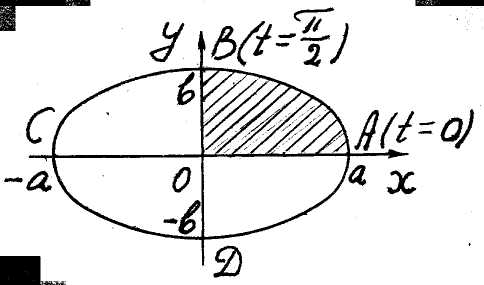
Ex. 10. Find the area of a figure bounded by an
ellipse
![]() (fig. 5).
(fig. 5).
It’s sufficient to find the quadruplicated area of the Fig. 5 part OAB of the figure.
The first way. From the equation of the ellipse
![]() ,
and so
,
and so

The second way. It’s better to pass to
parametric equations of the ellipse, na-mely
![]() 6.
In this case
6.
In this case

 .
.
Integration by parts
Theorem 5. If
functions
![]() are continuous with their derivatives on a segment
are continuous with their derivatives on a segment![]() ,
then the next formula (formula of
integration by parts) is true
,
then the next formula (formula of
integration by parts) is true
![]() ( 25 )
( 25 )
■To prove this formula it’s sufficient to integrate from a to b both parts of the identity
![]()
and
apply Newton-Leibniz formula for the integral of the expression
![]() ■
■
Ex. 11. Evaluate the definite integral
![]() .
.


![]()
Ex. 12. Find the area of a figure boun-ded by two
curves
![]() (see fig. 6).
(see fig. 6).
The curves
inter-sect at the
points
![]() and form a given figure
and form a given figure
![]() .
Its area is equal to the difference of the
areas of two curvilinear tra-
Fig. 6
peziums
.
Its area is equal to the difference of the
areas of two curvilinear tra-
Fig. 6
peziums
![]() .
.

![]() .
.
Ex. 13. Let
 .
Prove that
.
Prove that
![]() .
.
■

![]() ■
■
For example

 .
.
Ex. 14. Find the remainder
![]() of Taylor formula in Lagrange form.
of Taylor formula in Lagrange form.
Let, for example,
![]() ,
and
,
and
![]() .
.
By Lagrange formula
![]() .
.
Taking
![]() we get
we get
![]() ,
,
and
after integration over the segment
![]()
 Therefore
![]()
To get for any n we write
![]() ,
,
then
we put
![]() and integrate n times
over
.
As the result we’ll get
and integrate n times
over
.
As the result we’ll get
![]()