Lecture no. 23. Definite integral: additional questions

POINT 1. APPROXIMATE INTEGRATION

POINT 2. IMPROPER INTEGRALS

POINT 3. EULER Г-FUNCTION

Point 1. Approximate integration

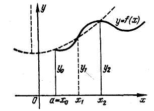
We’ll study the case of nonnegative function when a definite integral

represents the area of a curvilinear trapezium bounded by straight lines , , the Ox-axis and a graph of the function . The same results remain valid in general case.

Rectangular Formulas

A. We divide the segment into n equal parts of the length by points

.

Straight lines divide the curve into n parts . Let’s denote by

Fig. 1

the values of the function at the division points (see fig. 1)

a) Substituting every part of the curve by the segments of straight lines we substitute the curvilinear trapezium by the set of rectangles with total area

Therefore

( 1 )

b) Similarly, substituting every part of the curve by the segments of straight lines , we get

( 2 )

Absolute error of the formulas (1), (2) has the order 1/n, that is

.

c) Dividing the segment into 2n equal parts of the length by points

(fig. 2),

we substitute the curvilinear trapezium by the set of rectan- Fig.2 gles with bases 2h, altitudes and total area

Hence

( 3 )

Absolute error of the formula (3) has the order 1/n², that is

It means that the formula (3) is more exact than both (1) and (2).

Trapezium Formula

After dividing the segment into n equal parts

(fig. 3) we divide the graph of the function into n parts of the length by points

.

Fig. 3 Substituting every part of the graph by segments

we substitute the curvilinear trapezium by the set of trapeziums with total area

.

So we get the next approximate formula (trapezium formula) ,

( 4 )

Its absolute error has the order 1/n², that is

.

It means that the formulas (3) and (4) have the same order of exactness.

Simpson’s formula (parabolic formula)

Let’s divide (by points ) the segment into an even number 2n of equal parts of the length and let

be points of the curve corresponding to the division points (see fig. 4 for the case 2n = 6).

At first we draw a quadratic parabola

through points (see fig. 4, 5). One can prove that the area of the figure between the arc of the parabola and the segment of the Ox-axis Fig. 4 equals

,

and we can write

.

Fig. 5 Carrying out the same procedure on the point triplets …, we get

.

Finally we get Simpson’s formula for approximate integration

(5)

Simpson’s formula (5) is the most exact in comparison with (1) – (4). Indeed, its absolute error has the order 1/n⁴ that is

.

For example in the case n = 3, 2n = 6 (fig. 4) Simpson’s formula has the next form

.

Ex. 1. Calculate approximately the integral .

Let’s form the next table of values of the argument and the function:

i
0	0.0	0.00	0.0000
1	0.2	0.04	0.0400
2	0.4	0.16	0.1593
3	0.6	0.36	0.3523
4	0.8	0.64	0.5972
5	1.0	1.00	0.8415
6	1.2	1.44	0.9915
7	1.4	1.96	0.9249
8	1.6	2.56	0.5487

It corresponds to division of the segment into parts of the length

.

By the formula (1)

.

By the formula (2)

.

Using the formula (3) we take 2n = 8, n = 4, , and so

.

By the formula (4)

.

We’ll apply the formula (5) two times.

At first we divide the segment into 2n = 4 parts, , , , , , correspondingly , , , , , , and therefore

Dividing now the segment into 2n = 8 parts, , we have

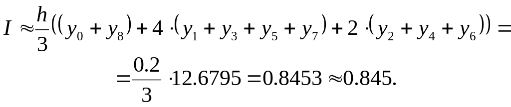
It’s useful to compare all these results with known approximate value of the same integral up to , namely

.