Lecture no.22. Applications of definite integral

POINT 1. PROBLEM – SOLVING SCHEMES. AREAS.

POINT 2. ARС LENGTH

POINT 3. VOLUMES

POINT 4. ECONOMIC APPLICATIONS

Point 1. Problem – solving schemes. Areas

There are two schemes for finding some quantity Q.

1) Setting integral sum, expression Q as the limit of this integral sum, that is in the form of a definite integral.

Ex. 1. See three problems in P. 1 of the 19-th lecture and corresponding formu-las (10), (11), (12) in P. 2 of the same lecture.

2) Finding an element (in fact the differential) dQ of Q and then expression Q as a sum of all these elements. This procedure leads by the other way to a definite integral to evaluate Q.

To illustrate this second scheme we’ll consider the same three problems as in the lecture No. 19.

Ex. 2. The area of a curvilinear trapezium

(fig. 1).

Element (differential) dS of the area S (the area of a hatched strip with the base on fig.1) equals

. Adding all these elements from a to b we get the re- Fig. 1 required area as known definite integral

( 1 )

Ex. 3. Produced quantity U of a factory during a time interval 0, T. Let be a labour productivity of the factory. An element of the produced quantity du-

ring an infinitely small time interval equals

.

Adding all these elements from 0 to T we get the sought produced quantity U, namely

( 2 )

Ex. 4. The length path L traveled by a material point during a time interval from t = 0 to t = T with the velocity .

An element dL of the length path traveled during an infinitely small time interval is equal to

,

and the sum of all these elements from 0 to T gives the length path L to be found

. ( 3 )

Certainly, results (1), (2), (3) coincide with those (10), (11), (12) of the preceding lecture.

Additional remarks about the areas of plane figures

a) The case of nonpositive function. The area of a figure

,

represented of the fig. 2, equals

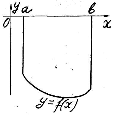Fig. 2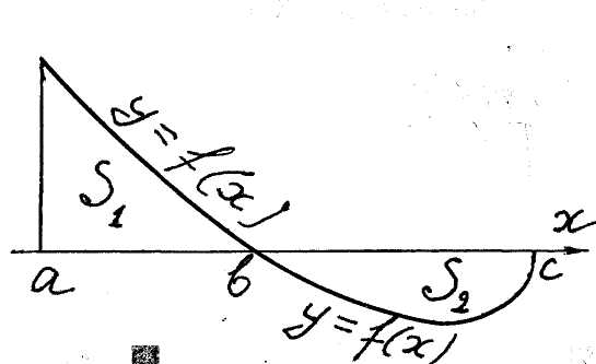

Fig. 3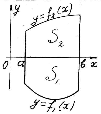

Fig. 4

. ( 4 )

b) The case when a function has different signs on various intervals. Let a function is nonnegative on the interval and nonpositive on the interval . The area of a corresponding figure, represented on the fig. 3, equals

. ( 5 )

c) The case when a figure lies between two curves. The area of a figure

,

represented on the fig. 4, equals

. ( 6 )

Ex. 5. Find the area enclosed by two curves (fig. 5).

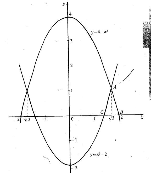Intersection points of the curves have abscises . The figure is symmetric about the Oy-axis; we may find double area of its right part.

Fig. 5 .

d) Figures oriented with respect to the Oy-axis. Areas of figures

(see fig. 6),

(see fig. 7),

(see fig. 8),

(see fig. 9),

are equal respectively

, ( 7 )

, ( 8 )

, ( 9 )

. ( 10 )

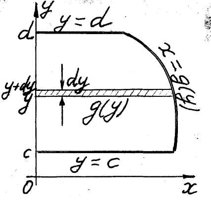Fig. 6

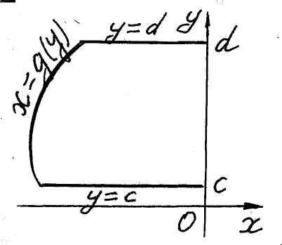Fig. 7

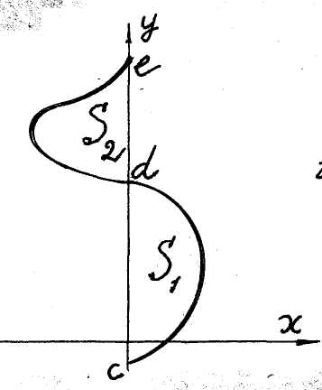Fig. 8

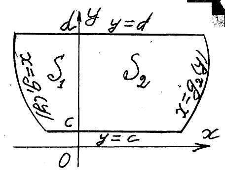Fig. 9

Ex. 6. Find the area of a figure bounded by curves (fig. 10).

It’s well to write the equations of the curves in the next form

and to utilize the formula (10). Fig. 10 By virtue of symmetry of the figure with respect to the Ox-axis

.

e) The case of parametrically represented curve.

Let, for example, be given a curvilinear trapezium

(fig. 1),

but a curve is determined by parametric equations ( for and for ). Fig. 11 To find the area of such the trapezium we change a variable in the integral (1), namely

.

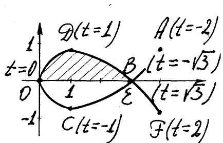
Ex. 7. Find the area of the loop of a curve (fig. 11).

To construct the curve point by point and to see the loop we equate to zero the expressions , and then form the next table

t	-2	-	-1	0	1		2
x	4	3	1	0	1	3	4
y		0	-	0		0	-
Point	A	B	C	O	D	E	F

From the fig. 11 we see that , and so

f) The area in polar coordinates.

Let be given a curvilinear sector (or a curvilinear triangle) that is a plane figure, bounded by two rays and a curve given in polar coordinates (fig. 12). Find the area of the sector.

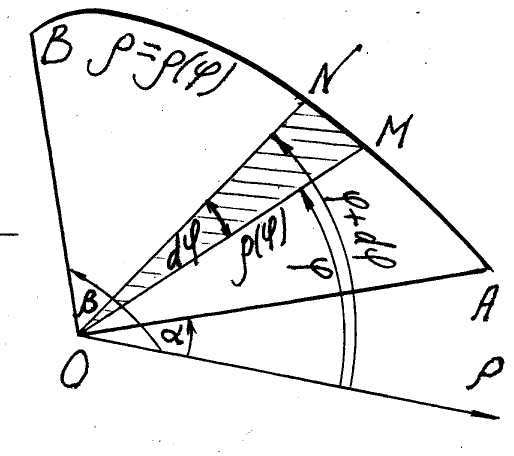Fig. 12

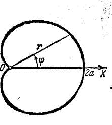Fig. 13

Fig. 14

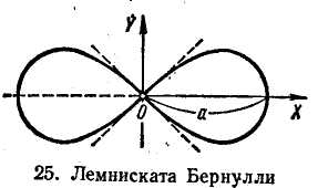
An element of the area is the area of a hatched circular sector with the radius and a central angle ,

.

Adding all these elements from to we get the area in question

. ( 11 )

Ex. 8. Find the area of a figure bounded by a cardioid (fig. 13).

Desired area equals the twofold area of upper part of the figure, which is a circular sector with the rays .

.

Ex. 9. Find the area of a figure bounded by Bernoulli lemniscate

.

The figure is symmetric with respect to the Ox-, Oy-axes and lies in the angles determined by the straight lines (fig. 14). Passing to polar coordinates , we write the equation of the lemniscate in more suitable form

Then we calculate the quadruplicated area of the circular sector bounded by the lemniscate and the rays . We obtain

.

POINT 2. ARС LENGTH

Let ˘ be an arc of some curve, and it’s necessary to find its length.

T he first method. We divide the arc ˜AB into n parts by points and inscribe the poly-gonal line in ˘AB (fig. 15). Let Fig. 15 ( 12 )

is the perimeter of the polygonal line and . If there exists the limit

( 13 )

it is called the length of the arc ˘AB.

Let an arc ˘ of a curve is determined in Cartesian coordinates by an equation

( 14 )

on a segment , and be the coordinates of the point , . In this case

,

and by Lagrange theorem there is a point such that

.

Denoting we get and therefore

.

Passage to the limit gives the desired arc length as a definite integral from a to b,

. ( 15 )

The arc length L exists if a function is continuous with the first derivative on the segment .

The second method. We find at first an element (or the differential) of desired arc length and then the arc length as the sum of all the elements.

By Pythagorean theorem and

. ( 16 )

For an arc ˘ determined by an equation (14)

,

and the sum of all the elements from a to b leads to the same formula (15).

If an arc ˘ of a curve is determined parametrically by equations

, ( 17 )

we have from (16)

,

and therefore

. ( 18 )

If an arc ˘ of a curve is given in polar coordinates by an equation

( 19 )

we pass to parametrical equations of the arc

( 20 )

and apply the formula (18). Since

the formula (18) gives

. ( 21 )

Ex. 10. Find the arc length of a curve for .

By virtue of the formula (15) we have

Ex. 11. Find the length of the loop of the curve (fig. 11).

By the formula (18)

.

Ex. 12. Find the length of the cardioid (fig. 13).

With the help of the formula (21)

Ex. 13. Find the length of an ellipse .

Parametrical equations of the ellipse and by the formula (18)

.

We can find only approximate value of L for given values of a and b because of a pri-mitive of the integrand is inexpressible in terms of elementary functions.

Ex. 14. Prove that the length of Bernoulli lemniscate (fig. 14) can be represented by the next integral

.