

Point 3. Improper double integrals. Poisson formula
We’ll limit ourselves to improper double integrals of the first kind that is integrals of continuous functions over unbounded domains. As such the domains we’ll consider: the first quadrant
![]() ,
,
an infinite rectangle
![]()
 and
the
-plane
and
the
-plane
![]() .
.
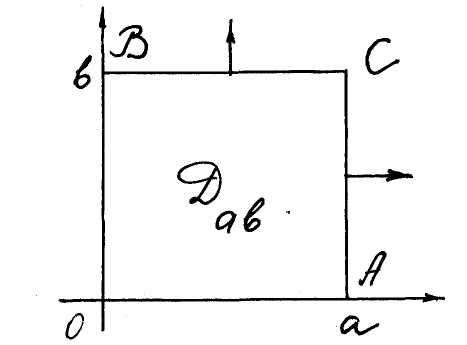
Let R
is the first quadrant and
![]() is a finite rectangle with sides a and
b (fig.
14). We define an improper integral
Fig. 14
over R as
the next limit
is a finite rectangle with sides a and
b (fig.
14). We define an improper integral
Fig. 14
over R as
the next limit

 .
.
As the corollary we get the formula of passing from a double integral to that repea-ting (the formula of interchange of integrations)
![]() .
( 8 )
.
( 8 )
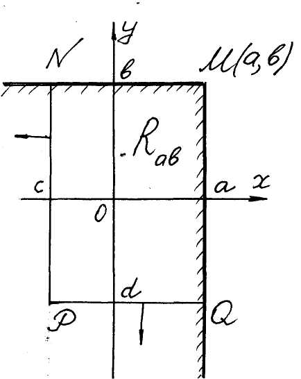
 An
improper integral over the rectangle
(see fig. 15) we define as the limit of the integral over a finite
rectangle
An
improper integral over the rectangle
(see fig. 15) we define as the limit of the integral over a finite
rectangle
![]() as
as
![]() ,
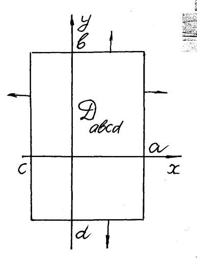
and an improper integral over the
-plane
we define as the limit of the inte-
Fig. 15
Fig. 16 gral over the same rectangle (fig. 16) as
,
and an improper integral over the
-plane
we define as the limit of the inte-
Fig. 15
Fig. 16 gral over the same rectangle (fig. 16) as
![]() ,
,
![]() and simultaneously
.
As the result we get the next two formulas
and simultaneously
.
As the result we get the next two formulas
 ,
( 9 )
,
( 9 )
![]() .
( 10 )
.
( 10 )
Ex. 6. Poisson
integrals
![]() .
( 11 )
.
( 11 )
■
Let’s integrate with respect to y
over the interval
![]() ,
,
![]()
![]() .
.
We’ve
proved that
![]() ,
and therefore
,
and therefore
![]() ■
■
Point 4. Double integral in polar coordinates
Let we study a double integral
![]()
over a domain D of the xOy-plane, and we pass to polar coordinates
![]() ,
( 12 )
,
( 12 )
coinciding
the pole O with
the origin
![]() and the polar axis
and the polar axis
![]() with
positive se-miaxis of the Ox-axis
of Cartesian coordinate system. The domain D
transforms into some domain
with
positive se-miaxis of the Ox-axis
of Cartesian coordinate system. The domain D
transforms into some domain
![]() of
the
of
the
![]() -plane
and the double integral passes in that over the do-main
.
-plane
and the double integral passes in that over the do-main
.
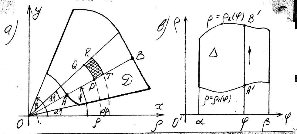 To
show up how the element dS
of the area changes we generate an element dD
of the domain D
by two circles of radii
To
show up how the element dS
of the area changes we generate an element dD
of the domain D
by two circles of radii
![]() centered at the origin
and by two rays starting
from the pole under angles
centered at the origin
and by two rays starting
from the pole under angles
![]() to the Ox-axis
(fig. 17 a). We can consider
Fig. 17 dD
as curvilinear rectangle PQRT
with the area
to the Ox-axis
(fig. 17 a). We can consider
Fig. 17 dD
as curvilinear rectangle PQRT
with the area
![]() .
.
Therefore
![]() ,
,
and the formula of passing to polar coordinates in a double integral can be written as
![]() .
( 13 )
.
( 13 )
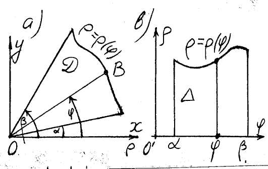
In applications we often meet the case of a domain D bounded by two rays
![]() ( 14 )
( 14 )
and two lines with polar equations
![]() ( 15 )
( 15 )
(fig. 17 a). One can describe such the domain by two double inequalities
![]() ,
( 16 )
,
( 16 )
whence
it follows that a domain Δ![]() (fig. 17 b), in which D transforms
after passage to polar coordinates, is that of the first type.
Therefore, by the formula (5)
(fig. 17 b), in which D transforms
after passage to polar coordinates, is that of the first type.
Therefore, by the formula (5)
 .
( 17 )
.
( 17 )
 If
a line
If
a line
![]() degenerates in the pole O we
get a curvilinear sector D bounded
by two rays
degenerates in the pole O we
get a curvilinear sector D bounded
by two rays
( 18 )
and a line with a polar equation
Fig. 18
![]() ( 19 )
( 19 )
(fig. 18 a). We describe it by inequalities
![]() ,
( 20 )
,
( 20 )
whence it follows that a domain Δ (fig. 18 b) is also that of the first type. Therefore, by the formula (5)
![]() .
( 21 )
.
( 21 )
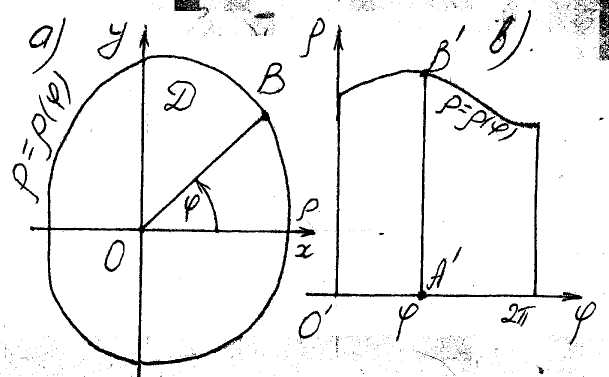 Let
a domain D contains
the pole O,
and every ray
Let
a domain D contains
the pole O,
and every ray
![]() intersects the boundary of the domain in unique point (fig. 19 a). If
(19) is its polar equation,
then
intersects the boundary of the domain in unique point (fig. 19 a). If
(19) is its polar equation,
then
![]() ( 22 )
Fig. 19 (fig. 19
b), and therefore
( 22 )
Fig. 19 (fig. 19
b), and therefore
![]() .
( 23 )
.
( 23 )
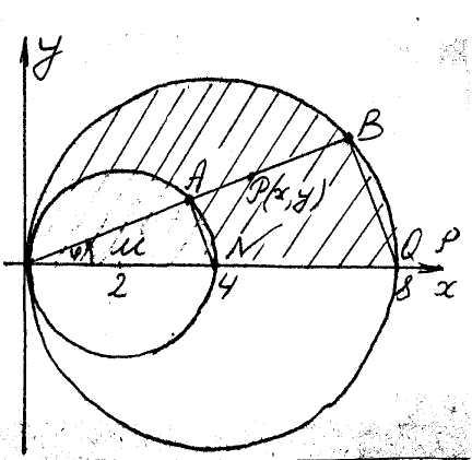 Ex.
7. Evaluate the mass of a plate D
containing betweem two curves
Ex.
7. Evaluate the mass of a plate D
containing betweem two curves
![]()
for
![]() (fig. 20), if its surface density
(fig. 20), if its surface density
![]() at any point
at any point
![]() is
proportional to the polar radius
Fig. 20
of OP this
point and equals 8 at the point
is
proportional to the polar radius
Fig. 20
of OP this
point and equals 8 at the point
![]() .
.
The surface density of the plate D
![]()
and by virtue of the mechanic sense of a double integral (see (3)) we have to calculate a double integral
![]() .
.
Compleating the squares we make sure that the
curves
![]() are circles with radii 2 and 4 and centres
are circles with radii 2 and 4 and centres
![]() correspondingly:
correspondingly:
![]() .
.
If we carry out the transition (12) to polare coordinates, we’ll get the polar equations of
![]()
and describe the domain D by two double inequalities
![]() .
.
Therefore by the formula (17)

 .
.
 Ex.
8. Find the area of a figure bounded by a curve (Bernoulli
lemniscate, fig. 21)
Ex.
8. Find the area of a figure bounded by a curve (Bernoulli
lemniscate, fig. 21)
![]() .
Fig. 21 We have studied this
curve in the Lecture 8, Point 2. Its polar equation is
.
Fig. 21 We have studied this
curve in the Lecture 8, Point 2. Its polar equation is
![]() .
.
Making use of the formula (2) we can write
![]()
where a domain D is the shaded area on the fig. 21. It’s evident that
![]() .
.
Hence in correspondence with the formula (20) the area in question equals
In generale case the substitution
![]() ,
when a domain D of
the plane xOy changes
in a domain
of a plane
,
when a domain D of
the plane xOy changes
in a domain
of a plane
![]() ,
there is the next formula
,
there is the next formula
![]() .
.