

Atomic physics (2005)
.pdf156 Doppler-free laser spectroscopy
16This is a convolution of the solution for a stationary atom with the velocity distribution (cf. Exercise 7.9).
17The cross-section only has a significant value near ω0, so taking the lower limit of the integration to be 0 (which is realistic) or −∞ (which is easy to evaluate) makes little di erence.
gH (ω − kv) ≡ δ (ω − ω0 − kv) that picks out atoms moving with velocity
v = |
ω − ω0 |
. |
(8.12) |
|
k |
|
|
Integration over v transforms f (v) into the Gaussian line shape function in eqn 8.4:16
gD (ω) = f (v) gH (ω − kv) dv . (8.13)
Thus since κ(ω) = N σ(ω) (from eqn 7.70) we find from eqn 8.11 that the cross-section for Doppler-broadened absorption is
σ (ω) = |
g2 |
|
π2c2 |
A21 gD (ω) . |
(8.14) |
g1 |
|
ω02 |
|||
|
|
|
|
Integration of gD (ω) over frequency gives unity, as in eqn 7.78 for homogeneous broadening. Thus both types of broadening have the same integrated cross-section, namely17
∞ |
|
g2 |
|
λ2 |
|
|
0 |
σ (ω) dω = |
|
|
0 |
A21 . |
(8.15) |
g1 |
4 |
The line broadening mechanisms spread this integrated cross-section out over a range of frequencies so that the peak absorption decreases as the frequency spread increases. The ratio of the peak cross-sections approximately equals the ratio of the line widths:
[σ(ω0)]Doppler |
|
gD (ω0) |
√ |
|
|
Γ |
|
|
|
|
|
||||||
|
= |
|
= |
π ln 2 |
|
|
. |
(8.16) |
[σ(ω0)] |
gH (ω0) |
∆ωD |
||||||
Homog |
|
|
|
|
|
|
|
|
√
The numerical factor π ln 2 = 1.5 arises in the comparison of a Gaussian to a Lorentzian. For the 3s–3p resonance line of sodium Γ/2π = 10 MHz and at room temperature ∆ωD/2π = 1600 MHz, so the ratio of the cross-sections in eqn 8.16 is 1/100. The Doppler-broadened gas gives less absorption, for the same N , because only 1% of the atoms interact with the radiation at the line centre—these are the atoms in the velocity class with v = 0 and width ∆v Γ/k. For homogeneous broadening all atoms interact with the light in the same way, by definition.
8.3.1Principle of saturated absorption spectroscopy
This method of laser spectroscopy exploits the saturation of absorption to give a Doppler-free signal. At high intensities the population di erence between two levels is reduced as atoms are excited to the upper level, and we account for this by modifying eqn 8.11 to read
∞
κ(ω) = |
{N1 (v) − N2 (v)} σabs (ω − kv) dv . |
(8.17) |
−∞
8.3 Saturated absorption spectroscopy 157
This is the same as the modification we made in going from eqn 7.70 to 7.72 but applied to each velocity class within the distribution. Here N1 (v) and N2 (v) are the number densities in levels 1 and 2, respectively, for atoms with velocities between v and v + dv. At low intensities almost all the atoms stay in level 1, so N1(v) N (v) has the Gaussian distribution in eqn 8.3 and N2 0, as illustrated in Fig. 8.3(a). For all intensities, the integral of the number densities in each velocity class equals the total number density in that level, i.e.
∞
N1 (v) dv = N1 , |
(8.18) |
−∞
and similarly for N2. The total number density N = N1 + N2.18
In saturated absorption spectroscopy the quantity N1(v) − N2(v) is a ected by interaction with a strong laser beam, as shown in Fig. 8.3(b) and Fig. 8.4 shows a typical experimental arrangement. The beam splitter divides the power of the laser beam between a weak probe and a stronger pump beam.19 Both these beams have the same frequency ω and the two beams go in opposite directions through the sample cell containing the atomic vapour. The pump beam interacts with atoms that have velocity v = (ω − ω0)/k and excites many of them into the upper level, as shown in Fig. 8.3(b). This is referred to as hole burning. The hole burnt into the lower-level population by a beam of intensity I has a width
∆ωhole = Γ 1 + |
I |
|
1/2 |
|
|
, |
(8.19) |
||||
Isat |
18This treatment of saturation is restricted to two-level atoms. Real systems with degeneracy are more di - cult to treat since, under conditions with signification saturation of the absorption, the atoms are usually not uniformly distributed over the sublevels (unless the light is unpolarized). Nevertheless, the expression N1(v) − g1N2(v)/g2 is often used for the di erence in population densities in a given velocity class.
19Normally, we have Iprobe Isat and
Isat.Ipump
equal to the power-broadened homogeneous width in eqn 7.88.
When the laser has a frequency far from resonance, |ω − ω0| ∆ωhole, the pump and probe beams interact with di erent atoms so the pump beam does not a ect the probe beam, as illustrated on the leftand
(a) |
(b) |
||||||||||||
|
|
|
|
|
|
|
|
|
|
|
|
|
Fig. 8.3 The saturation of absorption. |
|
|
|
|
|
|
|
|
|
|
|
|
|
(a) A weak beam does not significantly |
|
|
|
|
|
|
|
|
|
|
|
|
|
alter the number density of atoms in |
|
|
|
|
|
|
|
|
|
|
|
|
|
each level. The number density in the |
|
|
|
|
|
|
|
|
|
|
|
|
|
lower level N1(v) has a Gaussian dis- |
|
|
|
|
|
|
|
|
|
|
|
|
|
|
|
|
|
|
|
|
|
|
|
|
|
|
|
tribution of velocities characteristic of |
|
|
|
|
|
|
|
|
|
|
|
|
|
Doppler broadening of width ∆ωD/k. |
|
|
|
|
|
|
|
|
|
|
|
|
|
The upper level has a negligible popu- |
|
|
|
|
|
|
|
|
|
|
|
|
|
lation, N2(v) 0. (b) A high-intensity |
|
|
|
|
|
|
|
|
|
|
|
|
|
laser beam burns a deep hole—the pop- |
|
|
|
|
|
|
|
|
|
|
|
|
|
ulation di erence N1(v) − N2(v) tends |
|
|
|
|
|
|
|
|
|
|
|
|
|
to zero for the atoms that interact most |
|
|
|
|
|
|
|
|
|
|
|
|
|
strongly with the light (those with ve- |
|
|
|
|
|
|
|
|
|
|
|
|
|
locity v = (ω−ω0)/k). Note that N1(v) |
|
|
|
|
|
|
|
|
|
|
|
|
|
does not tend to zero: strong pumping |
|
|
|
|
|
|
|
|
|
|
|
|
|
of a two-level system never gives popu- |
|
|
|
|
|
|
|
|
|
|
|
|
|
lation inversion. This figure also shows |
|
|
|
|
|
|
|
|
|
|
|
|
|
clearly that Doppler broadening is in- |
|
|
|
|
|
|
|
|
|
|
|
|
|
homogeneous so that atoms interact in |
|
|
|
|
|
|
|
|
|
|
|
|
|
di erent ways within the radiation. |

158 Doppler-free laser spectroscopy
(a) |
|
|
Laser |
|
|
|
|
BS |
|
|
Probe |
Pump |
|
|
|
beam |
|
||
|
beam |
|
||
|
|
M1 |
||
|
|
|
|
|
|
|
|
Sample |
Detector |
(b) |
|
|
|
|
|
Signal without |
pump beam |
|
|
|
Signal with |
pump beam |
|
|
(c) |
} |
|
} |
} |
|
|
|
|
|
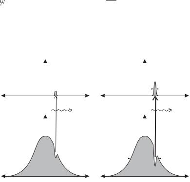
Fig. 8.4 (a) A saturated absorption spectroscopy experiment. The beam splitter BS, e.g. a piece of glass, divides the laser power between a weak probe and a stronger pump beam. The figure shows a finite angle of intersection between the weak probe beam and the stronger pump beam in the sample; this arrangement makes it straightforward to detect the probe beam after the cell but it leaves some residual Doppler broadening. Therefore saturated absorption experiments often have the pump and probe beams exactly counter-propagating and use a partially-reflecting mirror at M1 to transmit some of the probe beam to the detector (while still reflecting enough of the pump beam). (b) A plot of the probe intensity transmitted through the sample as a function of the laser frequency. With the pump beam blocked the experiment gives a simple Doppler-broadened absorption, but in the presence of the pump beam a narrow peak appears at the atomic resonance frequency. (c) The population densities of the two levels N1(v) and N2(v) as a function of velocity for three di erent laser frequencies: below, equal to, and above the atomic resonance, showing the e ect of the pump and probe beams.
8.3 Saturated absorption spectroscopy 159
right-hand sides of Fig. 8.4(c). Close to resonance, ω ω0, both beams interact with atoms in the velocity class with v 0, and the hole burnt by the pump beam reduces the absorption of the probe beam. Thus saturation of the absorption by the pump beam leads to a narrow peak in the intensity of the probe beam transmitted through the sample, as shown in Fig. 8.4(b). Normally, the pump beam has an intensity of about the saturation intensity Isat, so the saturated absorption peaks always have a line width greater than the natural width. The velocity class of atoms that interact with the light has a velocity spread ∆v = ∆ωhole/k.
This section shows how saturation spectroscopy picks out a signal from the atoms in the velocity class centred at v = 0 to give a signal at the atomic resonance frequency. It is the homogeneous broadening of these stationary atoms that determines the widths of the peaks. Exercise 8.8 goes through a detailed calculation of this width. Many experiments use this Doppler-free technique to give a stable reference, e.g. to set the laser frequency a few line widths below resonance in laser cooling experiments with the optical molasses technique (described in the next chapter).20
20Nowadays, inexpensive semiconductor diode lasers make saturation spectroscopy a feasible experiment in undergraduate teaching laboratories, using the alkali elements rubidium or caesium that have su cient vapour pressure at room temperature that a simple glass cell can be used as the sample (Wieman et al. 1999).
8.3.2Cross-over resonances in saturation spectroscopy
In a saturated absorption spectrum, peaks appear at frequencies midway between pairs of transitions that have energy levels in common (and a separation less than the Doppler width), e.g. for the three-level atom shown in Fig. 8.5(a). To explain these cross-over resonances we need to consider the situation shown in Fig. 8.5(b), where the pump beam burns two holes in the velocity distribution. These holes give rise to two peaks in the spectrum when the laser frequency corresponds to the frequencies of the two transitions—the ‘expected’ saturated absorption signals for these two transitions. However, an additional peak appears when the hole burnt by one transition reduces the absorption for the other transition. As illustrated by Fig. 8.5(b), the symmetry of this situation means that cross-overs occur exactly midway between two saturated absorption peaks. This property allows experimenters to identify the cross-overs in a saturated absorption spectrum (see the exercises at the end of this chapter), and these extra peaks do not generally cause confusion.
The spectral lines of atomic hydrogen have large Doppler widths because it is the lightest element, but physicists want to measure the energy levels of this simple atom precisely to test atomic physics theory and to determine the Rydberg constant.
Figure 8.6 shows a spectrum of the Balmer-α line (n = 2 to n = 3) that is limited by Doppler broadening. This red line of atomic hydrogen, at a wavelength of λ = 656 nm, has a Doppler width of ∆fD = 6 GHz at room temperature (Section 8.1); this is less than the 11 GHz interval between the j = 1/2 and 3/2 fine-structure levels in the n = 2 shell. Using the isotope deuterium (which has twice the atomic mass of hydrogen) in a discharge cooled to 100 K reduces the Doppler width to ∆fD = 2.3 GHz,21 where one factor arises from the mass and the other from the
21As calculated by scaling the value for hydrogen. The ratio of the Doppler
widths for H at T = 300 K and D at |
||||||
√ |
|
√ |
|
√ |
|
|
T = 100 K is |
6 = |
2 × 3. |
||||

160 Doppler-free laser spectroscopy
(a)
(b)
of probe |
detector |
Intensity |
beam at |
Cross-over
X
Fig. 8.5 The formation of a cross-over resonance. (a) A three-level atom with two allowed transitions at angular frequencies ω12 and ω13. (b) A cross-over resonance occurs at X, midway between two saturated absorption peaks corresponding to transitions at angular frequencies ω12 and ω13. At the cross-over the hole burnt by the pump beam acting on transition 1 ↔ 2 reduces the probe beam absorption on transition 1 ↔ 3, and vice versa.
22The expectation value of the spin– orbit interaction scales as 1/n3 (in eqn 2.56) and hence the splitting for n = 3 is 8/27 0.3 times that for n = 2.
temperature. This makes it possible to observe components separated by the 3.3 GHz interval between the j = 1/2 and 3/2 fine-structure levels in the n = 3 shell—see Figs 8.6(c) and 8.7(a).22 Structure on the scale of the 1 GHz corresponding to the Lamb shift cannot be resolved by conventional Doppler-limited techniques.
Figure 8.7 shows the spectacular improvement in resolution obtained with Doppler-free spectroscopy. The saturated absorption spectrum shown in Fig. 8.7(c) was obtained in a room-temperature discharge of

8.3 Saturated absorption spectroscopy 161
(a)
Free spectral range 


Frequency
(b)
D D
H H
Frequency
Free spectral range 


(c) 


 D D
D D
H H
Frequency
atomic hydrogen and part of the spectrum in Fig. 8.6(b) is shown for comparison.23 The saturated absorption technique gives clearly resolved peaks from the 2a and 2b transitions with a separation equal to the Lamb shift—the QED contributions shift the energy of the 2s 2S1/2 level upwards relative to 2p 2P1/2. Lamb and Retherford had measured this shift by a radio-frequency method using a metastable beam of hydrogen
Fig. 8.6 Spectroscopy of the Balmer-α line, carried out with an apparatus similar to that in Fig. 1.7(a), has a resolution limited by the Doppler e ect. (a) The transmission peaks of a pressurescanned Fabry–Perot ´etalon obtained with a highly-monochromatic source (helium–neon laser). The spacing of the peaks equals the free-spectral range of the ´etalon given by FSR = 1/2l = 1.68 cm−1, where l is the distance between the two highly-reflecting mirrors. The ratio of the FSR to the width of the peaks (FWHM) equals the finesse of the ´etalon, which is about 40 in this case. (The di erence in height of the two peaks in this trace of real data arises from changes in laser intensity over time.) In all the traces, (a) to (c), the ´etalon was scanned over two freespectral ranges. (b) The spectrum from a discharge of hydrogen, H, and deuterium, D, at room temperature. For each isotope, the two components have a separation approximately equal to the interval between the fine-structure levels with n = 2. This splitting is slightly larger than the Doppler width for hydrogen. The isotope shift between the hydrogen and deuterium lines is about 2.5 times larger than the free-spectral range, so that adjacent peaks for H and D come from di erent orders of the ´etalon. (The ´etalon length has been carefully chosen to avoid overlap whilst giving high resolution.) (c) The spectrum of hydrogen and deuterium cooled to around 100 K by immersing the discharge tube in liquid nitrogen. (The relative intensities change with discharge conditions.) The fine structure of the 3p configuration is not quite resolved, even for deuterium, but leads to observable shoulders on the left of each peak—the relevant energy levels are shown in Fig. 8.7. Courtesy of Dr John H. Sanders, Physics department, University of Oxford.
23The first saturated absorption spectrum of hydrogen was obtained by Professor Theodor H¨ansch and co-workers at Stanford University (around 1972). In those pioneering experiments the width of the observed peaks was limited by the bandwidth of the pulsed lasers used. Continuous-wave lasers have lower bandwidth.

162 Doppler-free laser spectroscopy
Fig. 8.7 Spectroscopy of the Balmer- α transition. (a) The levels with principal quantum numbers n = 2 and n = 3 and the transitions between them. Relativistic quantum mechanics (the Dirac equation) predicts that energies depend only on n and j, leading to the five transitions labelled 1 to 5 in order of decreasing strength (proportional to the square of the matrix element). In reality, some of these levels are not degenerate because of QED e ects, e.g. the Lamb shift between 2s 2S1/2 and 2p 2P1/2 that gives two components in transitions 2 and 3. Thus there are seven optical transitions (that were listed in Section 2.3.5). (The allowed transition between the 2s 2S1/2 and 2p 2P1/2 levels, and other radio-frequency transitions are not marked.) (b) The Doppler-broadened profile of the Balmer-α line in a room-temperature discharge containing atomic hydrogen shows only two clear components separated by about 10 GHz (slightly less than the fine-structure splitting of the 2p configuration—see the caption of Fig. 8.6). (c) The saturated absorption spectrum obtained with a continuous-wave laser. The Lamb shift between the 2a and 2b components is clearly resolved. The
level has a hyperfine splitting of 178 MHz and this leads to the double-peaked profile of 2a, 3a and the cross-over resonance X midway between them. (In addition to their relative positions, further evidence that peak X is the cross-over resonance between 2a and 3a comes from their similar line shape, which strongly indicates that they share a common level; the weak transition 3b is obscured.) Transition 4 is also seen on the far left and the cross-over resonance between 4 and 1 is just visible as a small bump on the base of peak 1. The scale gives the laser frequency relative to an arbitrary point (transition 1). Data shown in (c) was obtained by Dr John R. Brandenberger and the author.
(a)
(b)
Doppler-broadened |
profile of hydrogen |
|
|
|
|
|
|
5 |
4 |
1 |
3a |
3b |
2a 2b |
(c) |
|
|
|
|
|
Lamb shift |
Saturation |
|
|
|
|
|
|
spectrum |
|
|
|
X |
|
|
|
|
|
|
|
|
−5 |
0 |
5 |
10 |
15 |
|
Relative laser frequency (GHz) |
|
||

8.4 Two-photon spectroscopy 163
(atoms in 2s 2S1/2 level) but it was not resolved by optical techniques before the invention of Doppler-free laser spectroscopy.
8.4Two-photon spectroscopy
Two-photon spectroscopy uses two counter-propagating laser beams, as shown in Fig. 8.8. This arrangement has a superficial similarity to saturated absorption spectroscopy experiments (Fig. 8.4) but these two Doppler-free techniques di er fundamentally in principle. In two-photon spectroscopy the simultaneous absorption of two photons drives the atomic transition. If the atom absorbs one photon from each of the counter-propagating beams then the Doppler shifts cancel in the rest frame of the atom (Fig. 8.9(a)):
v |
& + ω $1 |
v |
& = 2ω . |
|
ω $1 + c |
− c |
(8.20) |
||
Laser |
Lens |
|
Sample |
Mirror |
|
|
|
|
Filter |
Beam splitter |
|
|
|
|
sends light |
|
Detector |
||
to calibration |
|
|||
Fig. 8.8 A two-photon spectroscopy experiment. The lens focuses light from the tunable laser into the sample and a curved mirror reflects this beam back on itself to give two counter-propagating beams that overlap in the sample. For this example, the photons spontaneously emitted after a two-photon absorption have di erent wavelengths from the laser radiation and pass through a filter that blocks scattered laser light. Usually, only one of the wavelengths corresponding to the allowed transitions at frequencies ω1i or ωi2 (in the cascade shown in Fig. 8.9(a)) reaches the detector (a photomultiplier or photodiode). The beam splitter picks o some laser light to allow measurement of its frequency by the methods discussed in Section 8.5.
(a)
Laboratory
frame:  Atom
Atom
Atom frame:
(b)2
1 
Fig. 8.9 (a) The atom has a component of velocity v along the axis of the laser beams (the light has frequency ω). The atoms sees an equal and opposite Doppler shift for each beam. So these shifts cancel out in the sum of the frequencies of the two counterpropagating photons absorbed by the atom (eqn 8.20). The sum of the frequencies does not depend on v so resonance occurs for all atoms when 2ω = ω12. (b) A two-photon transition between levels 1 and 2. The atom decays in two steps that each emit a single photon with frequencies ωi2 and ω1i .

164 Doppler-free laser spectroscopy
2
1
Fig. 8.10 A stimulated Raman transition between levels 1 and 2, via a virtual level. Level i is not resonantly excited in this coherent process.
When twice the laser frequency ω equals the atomic resonance frequency 2ω = ω12 all the atoms can absorb two photons; whereas in saturation spectroscopy the Doppler-free signal comes only from those atoms with zero velocity.
For the energy-level structure shown in Fig. 8.9(b) the atom decays in two steps that each emit a single photon (following the two-photon absorption). Some of these photons end up at the detector. A brief consideration of this cascade process illustrates the distinction between a two-photon process and two single-photon transitions. It would be possible to excite atoms from 1 to 2 using two laser beams with frequencies ωL1 = ω1i and ωL2 = ωi2 resonant with the two electric dipole transitions, but this two-step excitation has a completely di erent nature to the direct two-photon transition. The transfer of population via the intermediate level i occurs at the rate determined by the rates of the two individual steps, whereas the two-photon transition has a virtual intermediate level with no transitory population in i. (Equation 8.20 shows that to get a Doppler-free signal the two counter-propagating beams must have the same frequency.) This distinction between singleand two-photon transitions shows up clearly in the theory of these processes (see Section E.2 of Appendix E) and it is worthwhile to summarise some of the results here. Time-dependent perturbation theory gives the rate of transitions to the upper level induced by an oscillating electric field E0 cos ωt. The calculation of the rate of two-photon transitions requires second-order time-dependent perturbation theory. Resonant enhancement of the second-order process occurs when 2ω = ω12 but this still gives a rate which is small compared to an allowed single-photon transition. Therefore, to see any second-order e ects, the first-order terms must be far o resonance; the frequency detuning from the intermediate level ω − ω1i must remain large (of the same order of magnitude as ω1i itself, as drawn in the Fig. 8.9(b)). Two-photon absorption has many similarities with stimulated Raman scattering—a process of simultaneous absorption and stimulated emission of two photons via a virtual intermediate level, as shown in Fig. 8.10 (see Appendix E).
Finally, although the di erence between two sequential electric dipole transitions (E1) and a two-photon transition has been strongly emphasised above, these processes do link the same levels. So from the E1 selection rules (∆l = ±1 between levels of opposite parity) we deduce the two-photon selection rules: ∆l = 0, ±2 and no change of parity, e.g. s–s or s–d transitions.
Two-photon spectroscopy was first demonstrated on the 3s–4d transition of atomic sodium which has a line width dominated by the natural width of the upper level. The 1s–2s transition in atomic hydrogen has an extremely narrow two-photon resonance, and the line width observed in experiments arises from the various broadening mechanisms that we study in the next section.

Example 8.3 Two-photon spectroscopy of the 1s–2s transition in atomic hydrogen
The 1s–2s two-photon transition in atomic hydrogen has an intrinsic natural width of only 1 Hz because the 2s configuration is metastable. An atom in the 2s energy level has a lifetime of 1/8 s, in the absence of any external perturbations, since there are no p configurations of significantly lower energy (see Fig. 2.2).24 In contrast, the 2p configuration has a lifetime of only 1.6 ns because of the strong Lyman-α transition to the ground state (with a wavelength of 121.5 nm in the vacuum ultraviolet). This huge di erence in lifetimes of the levels in n = 2 gives an indication of the relative strengths of singleand two-photon transitions. The 1s–2s transition has an intrinsic quality factor of Q = 1015, calculated from the transition frequency 34 cR∞ divided by its natural width. To excite this two-photon transition the experiments required ultraviolet radiation at wavelength λ = 243 nm.25
Figure 8.11 shows a Doppler-free spectrum of the 1s–2s transition. A resolution of 1 part in 1015 has not yet been achieved because the various mechanisms listed below limit the experimental line width.
(a)Transit time Two-photon absorption is a nonlinear process26 with a rate proportional to the square of the laser beam intensity, I2 (see Appendix E). Thus to give a high signal experimenters focus the counter-propagating beams down to a small size in the sample, as indicated in Fig. 8.8. For a beam diameter of d = 0.5 mm transittime broadening gives a contribution to the line width of
|
∆ωtt |
|
u |
|
2200 m s−1 |
|
|
∆ftt = |
|
|
|
= |
|
= 4 MHz , |
(8.21) |
2π |
d |
5 × 10⁻⁴ m |
|||||
where u is a typical velocity for hydrogen atoms (see eqn 8.7).
(b)Collision broadening (also called pressure broadening) Collisions with other atoms, or molecules, in the gas perturb the atom (interacting with the radiation) and lead to a broadening and frequency shift of the observed spectral lines. This homogeneous broadening mechanism causes an increase in the line width that depends on the collision rate 1/τcoll, where τcoll is the average time between collisions. In a simple treatment, the homogeneous width of a transition whose natural width is Γ becomes ∆ωhomog = Γ+2/τcoll = Γ+2N σv, where σ is the collision cross-section and v is the mean relative velocity, as described by Corney (2000)—see also Loudon (2000) or Brooker (2003). The number density of the perturbing species N is proportional to the pressure. For the 1s–2s transition frequency the pressure broadening was measured to be 30 GHz/bar for hydrogen atoms in a gas that is mostly hydrogen molecules (H2), and this gives a major contribution to the line width of the signal shown in Fig. 8.11 of about 8 MHz (at the frequency of the ultraviolet radiation near 243 nm).27 Some further details are given in Exercise 8.7.
(c)Laser bandwidth The first two-photon experiments used pulsed lasers to give high intensities and the laser bandwidth limited the
8.4Two-photon spectroscopy 165
24The microwave transition from the 2s 2S1/2 level down to the 2p 2P1/2 level has negligible spontaneous emission.
25Such short-wavelength radiation cannot be produced directly by tunable dye lasers, but requires frequency doubling of laser light at 486 nm by secondharmonic generation in a nonlinear crystal (a process that converts two photons into one of higher energy). Thus the frequency of the laser light (at 486 nm) is exactly one-quarter of the 1s–2s transition frequency (when both the factors of 2 for the frequencydoubling process and two-photon absorption are taken into account); thus the laser light (at 486 nm) has a frequency very close to that of the Balmer- β line (n = 2 to n = 4) because the energies are proportional to 1/n2 in hydrogen.
26In contrast, single-photon scattering well below saturation is a linear process proportional to the intensity I. Saturated absorption spectroscopy is a nonlinear process.
27Collisions shift the 1s–2s transition frequency by −9 GHz/bar and this pressure shift is more troublesome for precision measurements than the broadening of the line (see Boshier et al. 1989 and McIntyre et al. 1989).