

Atomic physics (2005)
.pdf116 Hyperfine structure and isotope shift
(a) |
|
Source |
|
Polarizer |
|
Interaction |
|
|
Analyser |
Detector |
|||||||||||
|
|
|
|
|
|
||||||||||||||||
|
of atoms |
|
|
|
|
|
|
region |
|
|
|
|
|
|
|
|
|||||
|
A magnet |
|
|
B magnet |
|
||||||||||||||||
|
|
|
|
|
|
|
|
|
|
|
|
||||||||||
|
|
|
|
|
|
|
|
|
|
|
|
|
|
|
|
|
|
|
|
|
|
|
|
|
|
|
|
|
|
|
|
C region |
|
|
|
|
|
|
|
|
|||
|
|
Oven |
|
|
|
|
|
|
|
|
|
|
|
|
|
|
|
|
|
|
|
|
|
|
|
|
|
|
s |
|
|
|
|
|
|
|
|
|
D |
||||
|
|
|
|
|
|
|
|
|
|
|
|
|
|
|
|
|
|||||
|
|
|
|
|
|
|
|
|
|
|
|
r.f. |
|||||||||
|
|
|
|
|
|
|
|
|
|
||||||||||||
|
|
|
|
|
|
|
|
|
|
|
|
|
|
|
|||||||
|
|
|
|
|
|
|
|
|
|
|
|
|
|
|
|
|
|
|
|
|
|
|
|
|
|
|
|
|
|
|
|
|
|
|
|
|
|
|
|
|
|
|
|
|
|
|
|
|
|
|
|
|
|
|
|
|
|
|
|
|
|
|
|
|
|
|
|
|
|
|
|
|
|
|
|
|
|
|
|
|
|
|
|
|
|
|
|
|
|
|
|
|
|
|
|
|
|
|
|
|
|
|
|
|
|
|
|
|
|
|
|
|
|
|
|
|
|
|
|
|
|
|
|
|
|
|
|
|
|
|
|
|
|
|
|
|
|
|
|
|
|
|
|
|
|
|
|
|
|
|
|
|
|
|
|
|
|
|
|
|
|
|
|
|
|
|
|
|
|
|
|
|
|
|
|
|
|
|
|
|
|
|
|
|
|
|
|
|
|
|
|
|
|
|
|
|
|
|
|
|
|
|
|
|
|
|
|
|
|
|
|
|
|
|
|
|
|
|
|
|
|
|
|
|
|
|
|
|
|
|
|
|
|
|
|
|
|
|
|
|
|
(b) Oven
D
(c)
Oven

 D r.f.
(d) |
Detected |
Flop-out |
|
||
|
flux of |
|
|
atoms |
|
Fig. 6.14 (a) The magnetic resonance technique in an atomic beam. Atoms emerge from an oven and travel through the collimating slit ‘s’ to the detector. The deflection of atoms by the magnetic field gradient in the A and B regions depends on MJ , as indicated. (b) Atoms that stay in the same MJ state are refocused onto the detector when the A and B regions have gradients in opposite directions. (c) Resonant interaction with radio-frequency radiation in the C region can change the MJ quantum number, MJ = + 12 ↔ MJ = −21 , so that atoms no longer reach the detector. (In a real apparatus the C region may be up to several metres long.) This is known as the flop-out arrangement and gives a signal as in (d). Further details are given in the text and in Corney (2000).

6.4 Measurement of hyperfine structure 117
atomic-beam experiment are as follows.
•Atoms emerge from an oven to form an atomic beam in an evacuated chamber. The atoms have a mean free path much greater than the length of the apparatus (i.e. there are no collisions).
•The deflection of atoms in the A and B regions depends on MJ . If these two regions have magnetic field gradients in the same direction,
as indicated in Fig. 6.15, then atoms only reach the detector if their
MJ quantum number changes in the C region, i.e MJ = + 21 ↔ MJ = −21 . This is known as the flop-in arrangement.37
•As the atoms travel from A into the C region their state changes adiabatically to that in a low magnetic field as shown in Fig. 6.16 (and similarly as the field changes between the C and B regions). The transitions in the low-field region that can be observed are those that connect states with di erent values of MJ in the high-field regions, e.g. the transitions:
low frequency (∆F = 0):
F = 1, MF = 0 ↔ F = 1, MF = −1 with ∆E = gF µBB ; higher frequency (∆F = ±1):
F = 0, |
MF = 0 |
↔ |
F = 1, |
MF = 0 |
with |
∆E = A , |
F = 0, |
MF = 0 |
↔ |
F = 1, |
MF = 1 |
with |
∆E = A + gF µBB . |
In this example, the MF = 1 ↔ MF = 0 change between the Zeeman sub-levels of the upper F = 1 level cannot be detected, but this
37The flop-out arrangement is shown in Fig. 6.14.
(a)
Oven

 D r.f.
(b) Detected |
Flop-in |
|
flux of |
||
|
||
atoms |
|
Fig. 6.15 (a) The trajectories of atoms in an atomic-beam apparatus similar to that shown in Fig. 6.14, but magnetic field gradients in the A and B regions have the same direction. Atoms only reach the detector if their MJ quantum number is changed in the C region by the interaction with radio-frequency radiation. This is known as the flop-in arrangement and gives a signal as in (b).

118 Hyperfine structure and isotope shift
Fig. 6.16 The method of magnetic res- |
|
|
|||
onance in an atomic beam detects tran- |
|
|
|||
sitions that occur at low field (in the C |
|
|
|||
region shown in Fig. 6.14) which cause |
|
1 |
|||
a change in the quantum number MJ |
|
||||
at high field (A and B regions). For ex- |
|
|
|||
ample, an atom that follows the path |
|
0 |
|||
indicated by the dotted line may start |
|
||||
|
−1 |
||||
in the state MJ = + 21 , go adiabatically |
|
||||
into the state F = 1, MF = 0 in the |
|
|
|||
C region, where it undergoes a transi- |
|
|
|||
tion to the state with M |
F = |
−1 |
and |
|
0 |
|
1 |
|
|||
then end up in the state MJ |
= |
−2 |
|
||
in the B region (or it may follow the |
|
|
|||
same path in the opposite direction). A |
|
|
|||
strong magnetic field gradient (which is |
|
|
|||
associated with a high field) is required |
Low field |
High field |
|||
in the A and B regions to give an ob- |
|||||
servable deflection of the atomic trajec- |
C region |
A and B regions |
|||
tories. |
|
|
|
||
|
|
|
|
|
|
does not lead to any loss of information since the hyperfine-structure constant A and gF can be deduced from the other transitions.
These transitions at microwaveand radio-frequencies are clearly not electric dipole transitions since they occur between sub-levels of the ground configuration and have ∆l = 0 (and similarly for the maser). They are magnetic dipole transitions induced by the interaction of the oscillating magnetic field of the radiation with the magnetic dipole of the atoms. The selection rules for these M1 transitions are given in Appendix C.
38Such quantum metrology has been used to define other fundamental constants, with the exception of the kilogram which is still defined in terms of a lump of platinum kept in a vault in Paris.
39The next chapter gives a complete treatment of the interaction of atoms with radiation.
6.4.2Atomic clocks
An important application of the atomic-beam technique is atomic clocks, that are the primary standards of time. By international agreement the second is defined to be 9 192 631 770 oscillation periods of the hyperfine frequency in the ground state of 133Cs (the only stable isotope of this element). Since all stable caesium atoms are identical, precise measurements of this atomic frequency in the National Standards Laboratories throughout the world should agree with each other, within experimental uncertainties.38
The definition of the second is realised using the hyperfine frequency of the F = 3, MF = 0 ↔ F = 4, MF = 0 transition in caesium. This transition between two MF = 0 states has no first-order Zeeman shift, but even the second-order shift has a significant e ect at the level of precision required for a clock. The apparatus can be designed so that the dominant contribution to the line width comes from the finite interaction time τ as atoms pass through the apparatus (transit time). Fourier transform theory gives the line width as39
∆f |
1 |
= |
vbeam |
, |
(6.40) |
τ |
l |
6.4 Measurement of hyperfine structure 119
where vbeam is the typical velocity in the beam and l is the length of the interaction region. Therefore the atomic beams used as primary standards are made as long as possible. An interaction over a region 2 m long gives a line width of ∆f = 100 Hz.40 Thus the quality factor is f /∆f 108; however, the centre frequency of the line can be determined to a small fraction of the line width.41 As a result of many years of careful work at standards laboratories, atomic clocks have uncertainties of less than 1 part in 1014. This illustrates the incredible precision of radio-frequency and microwave techniques, but the use of slow atoms gives even higher precision, as we shall see in Chapter 10.42 There is a great need for accurate timekeeping for the synchronisation of global telecommunications networks, and for navigation both on Earth through the global positioning system (GPS) and for satellites in deep space.
The atomic-beam technique has been described here because it furnishes a good example of the Zeeman e ect on hyperfine structure, and it was also historically important in the development of atomic physics. The first atomic-beam experiments were carried out by Isador Rabi and he made numerous important discoveries. Using atomic hydrogen he showed that the proton has a magnetic moment of 2.8 µN, which was about three times greater than expected for a point-like particle (cf. the electron with µB, i.e. one unit of the relevant magnetic moment). This was the first evidence that the proton has internal structure. Other important techniques of radio-frequency spectroscopy such as optical pumping are described elsewhere, see Thorne et al. (1999) and Corney (2000).
40Caesium atoms have velocities of vCs = (3kBT /MCs)1/2 = 210 m s−1 at T = 360 K.
41In a normal experiment it is hard to measure the centre of a line with an uncertainty of better than one-hundredth
of the line width, i.e. a precision of only 1 in 1010 in this case.
42The hydrogen maser achieves a long interaction time by confining the atoms
in a glass bulb for τ 0.1 s to give a line width of order 10 Hz—the atoms bounce o the walls of the bulb without losing coherence. Thus masers can be more precise than atomic clocks but this does not mean that they are more accurate, i.e. the frequency of a given maser can be measured to more decimal places than that of an atomicbeam clock, but the maser frequency is shifted slightly from the hyperfine frequency of hydrogen by the e ect of collisions with the walls. This shift leads to a frequency di erence between masers that depends on how they were made. In contrast, caesium atomic clocks measure the unperturbed hyperfine frequency of the atoms. (The use of cold atoms improves the performance of both masers and atomic clocks—the above remarks apply to uncooled systems.)
Further reading
Further details of hyperfine structure and isotope shift including the electric quadrupole interaction can be found in Woodgate (1980). The discussion of magnetic resonance techniques in condensed matter (Blundell 2001) gives a useful complement to this chapter.
The classic reference on atomic beams is Molecular beams (Ramsey 1956). Further information on primary clocks can be found on the web sites of the National Physical Laboratory (for the UK), the National Institute of Standards and Technology (NIST, in the US), and similar sites for other countries. The two volumes by Vannier and Auduoin (1989) give a comprehensive treatment of atomic clocks and frequency standards.
120 Hyperfine structure and isotope shift
Exercises
(6.1) The magnetic field in fine and hyperfine structure
Calculate the magnetic flux density B at the centre of a hydrogen atom for the 1s 2S1/2 level and also for 2s 2S1/2.
Calculate the magnitude of the orbital magnetic field experienced by a 2p-electron in hydrogen (eqn 2.47).
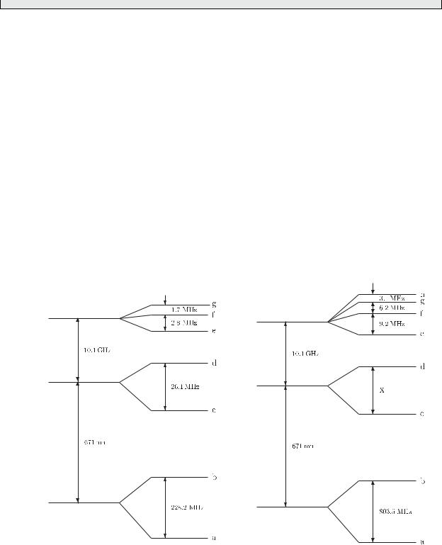
(6.2) Hyperfine structure of lithium
The figure shows the energy levels of lithium involved in the 2s–2p transitions for the two isotopes 6Li and 7Li. (The figure is not to scale.)
Explain in simple terms why the hyperfine splitting is of order me/Mp smaller than the finestructure splitting in the 2p configuration of lithium.
Explain, using the vector model or otherwise, why the hyperfine interaction splits a given J level into 2J + 1 hyperfine levels if J I and 2I + 1 levels if I J. Hence, deduce the nuclear spin of 6Li and give the values of the quantum numbers L, J and F for all its hyperfine levels. Verify that the
6Li
interval rule is obeyed in this case.
Determine from the data given the nuclear spin of 7Li and give the values of L, J and F for each of the hyperfine levels on the figure. Calculate the hyperfine splitting of the interval marked X.
(For the hyperfine levels a to d the parameter Anlj is positive for both isotopes.)
(6.3) Hyperfine structure of light elements
Use the approximate formula in eqn 6.17 to estimate the hyperfine structure in the ground states of atomic hydrogen and lithium. Comment on the di erence between your estimates and the actual values given for hydrogen in Section 6.1.1 and for Li in Exercise 6.2.
(6.4) Ratio of hyperfine splittings
The spin and magnetic moment of the proton are (1/2, 2.79µN ), of the deuteron (1, 0.857µN ) and of 3He (1/2, −2.13µN). Calculate the ratio of the ground-state hyperfine splittings of (a) atomic hydrogen and deuterium and (b) atomic hydrogen and the hydrogen-like ion 3He+.
7Li

Exercises for Chapter 6 121
(6.5) Interval for hyperfine structure
(a)Show that an interaction of the form A I · J leads to an interval rule, i.e. the splitting between two sub-levels is proportional to the total angular momentum quantum number F of the sub-level with the larger F .
(b)
III
Peak |
Position (GHz) |
Natural potassium is a mixture of 39K and 41K in |
a |
11.76 |
the ratio 14 : 1. Explain the origin of the struc- |
b |
10.51 |
ture, and deduce the nuclear spins and the ratio |
c |
8.94 |
of the magnetic moments of the two isotopes. |
d7.06
e4.86
f |
2.35 |
Energy |
|
|
|
The table gives the positions of the six peaks in the spectrum shown in Fig. 6.6 that were not assigned quantum numbers in Example 6.2. It is the hyperfine structure of the upper level (8D11/2) of the transition in the isotope 153Eu that determines the positions of these six peaks. What is the nuclear spin I of this isotope? Show that the spacing between these peaks obeys an interval rule and determine the quantum number F associated with each peak.
|
(c) For the isotope 151Eu, whose hyperfine struc- |
|
|
|
|
|
|||||||
|
|
|
|
|
|
||||||||
|
ture was analysed in Example 6.2, the lower |
|
|
|
|
|
|||||||
|
level of the transition has a hyperfine struc- |
(6.8) |
Zeeman e ect on HFS at all field strengths |
||||||||||
|
ture constant of A 8S7/2 = 20 MHz (mea- |
||||||||||||
|
|
The figure shows the hyperfine structure of the |
|||||||||||
|
sured by the method of magnetic resonance |
|
|||||||||||
|
|
|
87 |
|
|
||||||||
|
|
|
|
|
|
|
|
|
ground level (5s 2S1/2) of 37Rb (which has A/h = |
||||
|
in an atomic beam (Sandars and Woodgate |
|
3.4 GHz), as a function of the magnetic flux den- |
||||||||||
|
1960)). What is the hyperfine-structure con- |
|
|||||||||||
|
|
sity B. |
|||||||||||
|
stant of this 8S7/2 level for the isotope 153Eu, |
|
|||||||||||
|
|
|
|
|
|
||||||||
|
analysed in this exercise? |
|
|
(a) |
Deduce the nuclear spin of this isotope of ru- |
||||||||
(6.6) |
Interval for hyperfine structure |
|
|
|
bidium. |
||||||||
|
|
(b) |
What are the appropriate quantum numbers |
||||||||||
|
The 3d |
5 |
4s4p |
6 |
P7/2 level of |
55 |
Mn is split by hy- |
|
|||||
|
|
|
|
|
|
for the states in both strong and weak fields |
|||||||
|
perfine interaction into six levels that have sepa- |
|
|
||||||||||
|
|
|
(mark these on a copy of the figure)? |
||||||||||
|
rations 2599, 2146, 1696, 1258 and 838 MHz. De- |
|
|
||||||||||
|
|
|
|
|
|
||||||||
|
duce the nuclear spin of 55Mn and show that the |
|
(c) |
Show that in the weak-field regime the sepa- |
|||||||||
|
separations confirm your value. |
|
|
ration between states is the same in the upper |
|||||||||
(6.7) |
Hyperfine structure |
|
|
|
|
and lower hyperfine levels. |
|||||||
|
|
|
|
|
|
|
|||||||
|
When studied by means of high-resolution spectro- |
|
(d) |
In a strong field the energy of the states is |
|||||||||
|
scopy, the |
resonance line |
4s 2S1/2–4p 2P1/2 of |
|
|
given by eqn 6.33. Show that in this regime |
|||||||
|
naturally-occurring potassium consists of four |
|
|
the four uppermost states have the same sepa- |
|||||||||
|
components with spacings and intensity ratios as |
|
|
ration between them (marked ∆ on the figure) |
|||||||||
|
shown in the following diagram. |
|
|
as the four lower-lying states. |
|||||||||
122Hyperfine structure and isotope shift
(e)Define what is meant by a ‘strong field’ when considering hyperfine structure. Give an approximate numerical value for the magnetic field at which the cross-over from the weakfield to the strong-field regime occurs in this example.
(6.9) Isotope shift
Estimate the contributions to the isotope shift between 8537Rb and 8737Rb that arise from the mass and volume e ects for the following transitions:
trons has a kinetic energy T given by
|
|
|
N |
|
|
|
T = |
pN2 |
+ |
i |
pi2 |
, |
|
2MN |
=1 |
2me |
||||
|
|
|
||||
|
|
|
|
|
where pN is the momentum of the nucleus and pi is the momentum of the ith electron. The total of these momenta is zero in the centre-of-mass frame of the atom:
N
pN + pi = 0 .
|
(a) 5s–5p at a wavelength of 790 nm; and |
|
i=1 |
|
|
Use this equation to express T in terms of elec- |
|
|
(b) 5p–7s at a wavelength of 730 nm. |
|
tronic momenta only. |
|
Estimate the total isotope shift for both transi- |
|
Answer the following for either (a) a lithium atom |
|
|
(with N = 3) or (b) the general case of a multi- |
|
|
tions, being careful about the sign of each contri- |
|
|
|
|
electron atom with a nucleus of finite mass (i.e. |
|
|
bution. |
|
|
|
|
any real non-hydrogenic atom). Find the kinetic- |
|
(6.10) |
Volume shift |
|
|
|
energy terms that are me/MN times the main |
||
|
Calculate the contribution of the finite nuclear size |
|
|
|
e ect to the Lamb shift between the 2p 2P1/2 and |
|
contribution: a normal mass e ect (cf. eqn 6.21) |
|
|
and a specific mass e ect that depends on prod- |
|
|
2s 2S1/2 levels in atomic hydrogen (using the infor- |
|
|
|
|
ucts of the momenta pi · pj . |
|
|
mation in Section 6.2.2). The measured value of |
(6.13) |
|
|
the proton charge radius has an uncertainty of 1% |
Muonic atom |
|
|
|
A muon of mass mµ = 207me is captured by an |
|
|
and the Lamb shift is about 1057.8 MHz. What |
|
|
|
|
atom of sodium (Z = 11). Calculate the radius of |
|
|
is the highest precision with which experimental |
|
|
|
|
the muon’s orbit for n = 1 using Bohr theory and |
|
|
measurement of the Lamb shift can test quantum |
|
|
|
|
explain why the atomic electrons have little influ- |
|
|
electrodynamics (expressed as parts per million)? |
|
|
|
|
ence on the energy levels of the muonic atom. Cal- |
|
(6.11) |
Isotope shift |
|
|
|
culate the binding energy of the muon for n = 1. |
||
|
Estimate the relative atomic mass A for which the |
|
|
|
|
Determine the volume e ect on the 1s–2p transi- |
|
|
volume and mass e ect give a similar contribution |
|
|
|
|
tion in this system; express the di erence between |
|
|
to the isotope shift for n 2 and a visible tran- |
|
|
|
|
the frequency of the transition for a nucleus with |
|
|
sition. |
|
a radius rN (given by eqn 6.25) and the theoretical |
|
|
|
|
(6.12) |
Specific mass shift |
|
frequency for rN = 0 as a fraction of the transition |
|
An atom with a nucleus of mass MN and N elec- |
|
frequency. |
Web site:
http://www.physics.ox.ac.uk/users/foot
This site has answers to some of the exercises, corrections and other supplementary information.

The interaction of atoms
with radiation |
7 |
|
To describe the interaction of a two-level atom with radiation we shall use a semiclassical treatment, i.e. the radiation is treated as a classical electric field but we use quantum mechanics to treat the atom. We shall calculate the e ect of an oscillating electric field on the atom from first principles and show that this is equivalent to the usual time-dependent perturbation theory (TDPT) summarised by the golden rule (as mentioned in Section 2.2). The golden rule only gives the steady-state transition rate and therefore does not describe adequately spectroscopy experiments with highly monochromatic radiation, e.g. radio-frequency radiation, microwaves or laser light, in which the amplitudes of the quantum states evolve coherently in time. In such experiments the damping time may be less than the total measurement time so that the atoms never reach the steady state.
From the theory of the interaction with radiation, we will be able to find the conditions for which the equations reduce to a set of rate equations that describe the populations of the atomic energy levels (with a steady-state solution). In particular, for an atom illuminated by broadband radiation, this approach allows us to make a connection with Einstein’s treatment of radiation that was presented in Chapter 1; we shall find the Einstein B coe cient in terms of the matrix element for the transition. Then we can use the relation between A21 and B21 to calculate the spontaneous decay rate of the upper level. Finally, we shall study the roles of natural broadening and Doppler broadening in the absorption of radiation by atoms, and derive some results needed in later chapters such as the a.c. Stark shift.
7.1Setting up the equations 123
7.2The Einstein B
coe cients |
126 |
7.3Interaction with monochromatic radiation 127
7.4 |
Ramsey fringes |
132 |
7.5 |
Radiative damping |
134 |
7.6 |
The optical absorption |
|
|
cross-section |
138 |
7.7 |
The a.c. Stark e ect or |
|
|
light shift |
144 |
7.8 |
Comment on |
|
|
semiclassical theory |
145 |
7.9 |
Conclusions |
146 |
Further reading |
147 |
|
Exercises |
148 |
|
7.1 Setting up the equations
We start from the time-dependent Schr¨odinger equation1 |
|
1The operators do not have hats so |
||
|
|
|
|
ˆ |
i |
∂Ψ |
= HΨ . |
(7.1) |
H ≡ H, as previously. |
|
|
|||
|
∂t |
|
|
|
The Hamiltonian has two parts, |
|
|
||
H = H0 + HI (t) . |
(7.2) |
|
||
That part of the Hamiltonian that depends on time, HI (t), describes the interaction with the oscillating electric field that perturbs the eigen-

124 The interaction of atoms with radiation
2Note that E0 cos (ωt) is not replaced by a complex quantity E0e−iωt, because a complex convention is built into quantum mechanics and we must not confuse one thing with another.
3This dipole approximation holds when the radiation has a wavelength greater than the size of the atom, i.e. λ a0, as discussed in Section 2.2.
4Section 2.2 on selection rules shows how to treat other polarizations.
functions of H0; the unperturbed eigenvalues and eigenfunctions of H0 are just the atomic energy levels and wavefunctions that we found in previous chapters. We write the wavefunction for the level with energy En as
Ψn (r, t) = ψn (r) e−iEnt/ . |
(7.3) |
For a system with only two levels, the spatial wavefunctions satisfy
H0ψ1 (r) = E1ψ1 (r) ,
(7.4)
H0ψ2 (r) = E2ψ2 (r) .
These atomic wavefunctions are not stationary states of the full Hamiltonian, H0 + HI (t) , but the wavefunction at any instant of time can be expressed in terms of them as follows:
Ψ (r, t) = c1 (t) ψ1 (r) e−iE1t/ + c2 (t) ψ2 (r) e−iE2t/ , |
(7.5) |
or, in concise Dirac ket notation (shortening c1 (t) to c1, ω1 = E1/ , etc.),
Ψ (r, t) = c1 |1 e−iω1t + c2 |2 e−iω2t . |
(7.6) |
Normalisation requires that the two time-dependent coe cients satisfy
|c1|2 + |c2|2 = 1 . |
(7.7) |
7.1.1Perturbation by an oscillating electric field
The oscillating electric field E = E0 cos (ωt) of electromagnetic radiation produces a perturbation described by the Hamiltonian
HI (t) = er · E0 cos (ωt) . |
(7.8) |
This corresponds to the energy of an electric dipole −er in the electric field, where r is the position of the electron with respect to the atom’s centre of mass.2 Note that we have assumed that the electric dipole moment arises from a single electron but the treatment can easily be generalised by summing over all of the atom’s electrons. The interaction mixes the two states with energies E1 and E2. Substitution of eqn 7.6 into the time-dependent Schr¨odinger eqn 7.1 leads to
. |
= Ω cos (ωt) e−iω0tc2 , |
|
|
||||
|
ic.1 |
|
(7.9) |
||||
|
ic2 |
= Ω cos (ωt) eiω0tc1 , |
|
(7.10) |
|||
where ω0 = (E2 − E1) / and the Rabi frequency Ω is defined by |
|
||||||
|
|
|
e |
|
|
|
|
Ω = |
1|er · E0 |2 |
= |
|
|
ψ1 (r) r · E0 ψ2 |
(r) d3r . |
(7.11) |
|
|
||||||
The electric field has almost uniform amplitude over the atomic wavefunction so we take the amplitude |E0| outside the integral.3 Thus, for radiation linearly polarized along the x-axis, E = |E0|ex cos (ωt), we obtain4

Ω = |
eX12|E0| |
, |
(7.12) |
|
|
||||
|
|
|
||
where |
|
|
|
|
X12 = 1|x |2 . |
(7.13) |
|||
To solve the coupled di erential equations for c1 (t) and c2 (t) we need to make further approximations.
7.1.2The rotating-wave approximation
When all the population starts in the lower level, c1 (0) = 1 and c2 (0) = 0, integration of eqns 7.9 and 7.10 leads to
c1 (t) = 1 , |
|
|
|
|
|
|
|
|
|
|
||
|
Ω |
1 |
|
exp [i(ω0 + ω)t] |
1 |
|
exp [i(ω0 |
ω)t] |
(7.14) |
|||
c2 (t) = |
|
|
|
− |
|
+ |
|
− |
− |
|
. |
|
2 |
|
|
|
ω0 + ω |
|
|
ω0 − ω |
|
||||
This gives a reasonable first-order approximation while c2 (t) remains small. For most cases of interest, the radiation has a frequency close to the atomic resonance at ω0 so the magnitude of the detuning is small, |ω0 − ω| ω0, and hence ω0 + ω 2ω0. Therefore we can neglect the term with denominator ω0 + ω inside the curly brackets. This is the rotating-wave approximation.5 The modulus-squared of the co-rotating term gives the probability of finding the atom in the upper state at time t as
(7.15)
or, in terms of the variable x = (ω − ω0)t/2,
2 |
|
1 |
|Ω| |
2 |
|
2 sin2 x |
|
||
|c2 (t)| |
= |
|
|
t |
|
|
. |
(7.16) |
|
4 |
|
x2 |
|||||||
The sinc function (sin x) /x has a maximum at x = 0, and the first minimum occurs at x = π or ω0 − ω = ±2π/t, as illustrated in Fig. 7.1; the frequency spread decreases as the interaction time t increases.
7.1 Setting up the equations 125
5This is not true for the interaction of atoms with radiation at 10.6 µm from a CO2 laser. This laser radiation has a frequency closer to d.c. than to the resonance frequency of the atoms, e.g. for rubidium with a resonance transition in the near infra-red (780 nm) we find that ω0 15ω, hence ω0 +ω ω0 −ω. Thus the counter-rotating term must be kept. The quasi-electrostatic traps (QUEST) formed by such long wavelength laser beams are a form of the dipole-force traps described in Chapter 10.
Fig. 7.1 The excitation probability function of the radiation frequency has a maximum at the atomic resonance. The line width is inversely proportional to the interaction time. The function sinc2 also describes the Fraunhofer diffraction of light passing through a single slit—the di raction angle decreases as the width of the aperture increases. The mathematical correspondence between these two situations has a natural explanation in terms of Fourier transforms.