

Atomic physics (2005)
.pdf86 The LS-coupling scheme
Fig. 5.8 The jj-coupling scheme. The spin–orbit interaction energy is large compared to the Ere. (Cf. Fig. 5.4 for the LS-coupling scheme.)
12In both of these cases we assume an isolated configuration, i.e. that the energy separation of the di erent configurations in the central field is greater than the perturbation produced by either Es−o or Ere.
In summary, the conditions for LS- and jj-coupling are as follows:12
LS-coupling scheme: Ere Es−o , jj-coupling scheme: Es−o Ere .
5.3Intermediate coupling: the transition between coupling schemes
In this section we shall look at examples of angular momentum coupling schemes in two-electron systems. Figure 5.9 shows energy-level diagrams of Mg and Hg and the following example looks at the structure of these atoms.
Example 5.1
3s3p, Mg 6s6p, Hg
2.1850 3.76
2.1870 3.94
2.1911 4.40
3.5051 5.40
The table gives the energy levels, in units of 106 m−1 measured from the ground state, for the 3s3p configuration in magnesium (Z = 12) and 6s6p in mercury (Z = 80). We shall use these data to identify the levels and assign further quantum numbers.
For an sp configuration we expect 1P and 3P terms. In the case of magnesium we see that the spacings between the three lowest levels are 2000 m−1 and 4100 m−1; these are close to the 1 to 2 ratio expected from the interval rule for the levels with J = 0, 1 and 2 that arise from the triplet. The LS-coupling scheme gives an accurate description because
5.3 Intermediate coupling: the transition between coupling schemes 87
0
−1
−2
−3
−4
−5
−6
−7
−8
−9
−10
−11
H |
|
|
|
|
|
|
|
|
|
|
|
|
|
He |
|
|
|
|
|
|
|
|
|
|
|
|
|
|
Mg |
|
|
|
|
|
|
|
|
|
|
|
|
|
|
|
|
|
|
|
|
|
|
Hg |
|
|
|
|
|
|
|
Complex |
|||||||||||||||
|
|
|
|
|
|
|
|
|
|
|
|
|
|
|
|
|
|
|
|
|
|
|
|
|
|
|
|
|
|
|
|
|
|
|
|
|
|
|
|
|
|
|
|
|
|
|
|
|
|
|
|
|
|
|
|
|
|
|
|
|
|
|
|
|
|
|
|
|
|
|
|
terms |
|||
|
9 |
|
|
|
|
|
|
|
|
|
|
|
|
|
|
|
|
|
|
|
|
|
|
|
|
|
|
|
|
|
|
|
|
|
|
|
|
|
|
|
|
|
|
|
|
|
|
|
|
|
|
|
|
|
|
|
|
|
|
|
|
|
|
|
|
|
|
|
|
|
|
|
|
|
|
|
|
|
|
|
|
|
|
|
|
|
|
|
|
|
|
|
|
|
|
|
|
|
|
|
|
|
|
|
|
|
|
|
|
|
|
|
|
|
|
|
|
|
|
|
|
|
|
|
|
|
|
|
|
|
|
|
|
|
|
|
|
|
|
|
|
|
|
|
|
|
|
|
|
|
|
|
|
|
|
|
|
|
|
|
|
|
|
|
|
|
|
|
|
|
|
|
|
|
|
|
|
|
|
|
|
|
|
|
|
|
|
|
|
|
|
|
|
|
|
|
|
|
|
|
|
|
|
|
|
|
|
|
|
|
|
|
|
|
|
|
|
|
|
|
|
|
|
|
|
|
|
|
87 |
|
|
|
|
|
|
|
|
|
|
|
|
|
|
|
|
|
|
|
|
|
|
|
|
|
|
|
|
|
|
|
|
|
|
|
|
|
|
|
|
|
|
|
|
|
|
|
|
|
|
|
|
|
|
|
|
|
|
|
|
|
|
|
|
|
|
|
|
|
|
|
|
|
|
|
6 |
|
|
|
|
|
|
|
|
|
|
|
|
|
|
|
|
|
|
|
|
|
|
|
|
|
|
|
|
|
|
|
|
|
|
|
|
|
|
|
|
|
|
|
|
|
|
|
|
|
|
|
|
|
|
|
|
|
|
|
|
|
|
|
|
|
|
|
|
|
|
|
|
|
|
|
5 |
|
|
|
|
|
|
|
|
|
|
|
|
|
|
|
|
|
|
|
|
|
|
|
|
|
|
|
|
|
|
|
|
|
|
|
|
|
|
|
|
|
|
|
|
|
|
|
|
|
|
|
|
|
|
|
|
|
|
|
|
|
|
|
|
|
|
|
|
|
|
|
|
|
|
|
4 |
|
|
|
|
|
|
|
|
|
|
|
|
|
|
|
|
|
|
|
|
|
|
|
|
|
|
|
|
|
|
|
|
|
|
|
|
|
|
|
|
|
|
|
|
|
|
|
|
|
|
|
|
|
|
|
|
|
|
|
|
|
|
|
|
|
|
|
|
|
|
|
|
|
|
|
3 |
|
|
|
|
|
|
|
|
|
|
|
|
|
|
|
|
|
|
|
|
|
|
|
|
|
|
|
|
|
|
|
|
|
|
|
|
|
|
|
|
|
|
|
|
|
|
|
|
|
|
|
|
|
|
|
|
|
|
|
|
|
|
|
|
|
|
|
|
|
|
|
|
|
|
|
|
|
|
|
|
|
|
|
|
|
|
|
|
|
|
|
|
|
|
|
|
|
|
|
|
|
|
|
|
|
|
|
|
|
|
|
|
|
|
|
|
|
|
|
|
|
|
|
|
|
|
|
|
|
|
|
|
|
|
|
|
|
|
|
|
|
|
|
|
|
|
|
|
|
|
|
|
|
|
|
|
|
|
|
|
|
|
|
|
|
|
|
|
|
|
|
|
|
|
|
|
|
|
|
|
|
|
|
|
|
|
|
|
|
|
|
|
|
|
|
|
|
|
|
|
|
|
|
|
|
|
|
|
|
|
|
|
|
|
|
|
|
|
|
|
|
|
|
|
|
|
|
|
|
|
|
|
|
|
|
|
|
|
|
|
|
|
|
|
|
|
|
|
|
|
|
|
|
|
|
|
|
|
|
|
|
|
|
|
|
|
|
|
|
|
|
|
|
|
|
|
|
|
|
|
|
|
|
|
|
|
|
|
|
|
|
|
|
|
|
|
|
|
|
|
|
|
|
|
|
|
|
|
|
|
|
|
|
|
|
|
|
|
|
|
|
|
|
|
|
|
|
|
|
|
|
|
|
|
|
|
|
|
|
|
|
|
|
|
|
|
|
|
|
|
|
|
|
|
|
|
|
|
|
|
|
|
|
|
|
|
|
|
|
|
|
|
|
|
|
|
|
|
|
|
|
|
|
|
|
|
|
|
|
|
|
|
|
|
|
|
|
|
|
|
|
|
|
|
|
|
|
|
|
|
|
|
|
|
|
|
|
|
|
|
|
|
|
|
|
|
|
|
|
|
|
|
|
|
|
|
|
|
|
|
|
|
|
|
|
|
|
|
|
|
|
|
|
|
|
|
|
|
|
|
|
|
|
|
|
|
|
|
|
|
|
|
|
|
|
|
|
|
|
|
|
|
|
|
|
|
|
|
|
|
|
|
|
|
|
|
|
|
|
|
|
|
|
|
|
|
|
|
|
|
|
|
|
|
|
|
|
|
|
|
|
|
|
|
|
|
|
|
|
|
|
|
|
|
|
|
|
|
|
|
|
|
|
|
|
|
|
|
|
|
|
|
|
|
|
|
|
|
|
|
|
|
|
|
|
|
|
|
|
|
|
|
|
|
|
|
|
|
|
|
|
|
|
|
|
|
|
|
|
|
|
|
|
|
|
|
|
|
|
|
|
|
|
|
|
|
|
|
|
|
|
|
|
|
|
|
|
|
|
|
|
|
|
|
|
|
|
|
|
|
|
|
|
|
|
|
|
|
|
|
|
|
|
|
|
|
|
|
|
|
|
|
|
|
|
|
|
|
|
|
|
|
|
|
|
|
|
|
|
|
|
|
|
|
|
|
|
|
|
|
|
|
|
|
|
|
|
|
|
|
|
|
|
|
|
|
|
|
|
|
|
|
|
|
|
|
|
|
|
|
|
|
|
|
|
|
|
|
|
|
|
|
|
|
|
|
|
|
|
|
|
|
|
|
|
|
|
|
|
|
|
|
|
|
|
|
|
|
|
|
|
|
|
|
|
|
|
|
|
|
|
|
|
|
|
|
|
|
|
|
|
|
|
|
|
|
|
|
|
|
|
|
|
|
|
|
|
|
|
|
|
|
|
|
|
|
|
|
|
|
|
|
|
|
|
|
|
|
|
|
|
|
|
|
|
|
|
|
|
|
|
|
|
|
|
|
|
|
|
|
|
|
|
|
|
|
|
|
|
|
|
|
|
|
|
|
|
|
|
|
|
|
|
|
|
|
|
|
|
|
|
|
|
|
|
|
|
|
|
|
|
|
|
|
|
|
|
|
|
|
|
|
|
|
|
|
|
|
|
|
|
|
|
|
|
|
|
|
|
|
|
|
|
|
|
|
|
|
|
|
2
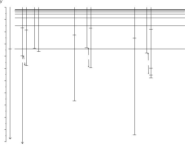
Fig. 5.9 The terms of helium, magnesium and mercury are plotted on the same energy scale (with hydrogen on the left for comparison). The fine structure of the lighter atoms is too small to be seen on this scale and the LS-coupling scheme gives a very accurate description. This scheme gives an approximate description for the low-lying terms of mercury even though it has a much larger fine structure, e.g. for the 6s6p configuration the Ere > Es−o but the interval rule is not obeyed because the spin–orbit interaction is not very small compared to the residual electrostatic interaction. The 1s2 configuration of helium is not shown; it has a binding energy of −24.6 eV (see Fig. 3.4). The 1s2s and 1s2p configurations of helium lie close to the n = 2 shell in hydrogen, and similarly the 1s3l configurations lie close to the n = 3 shell. In magnesium, the terms of the 3snf configurations have very similar energies to those in hydrogen, but the di erences get larger as l decreases. The energies of the terms in mercury have large di erences from the hydrogen energy levels. Much can be learnt by carefully studying this term diagram, e.g. there is a 1P term which has similar energy in the three configurations: 1s2p, 3s3p and 6s6p in He, Mg and Hg, respectively—thus the e ective quantum number n is similar despite the increase in n. Complex terms arise when both valence electrons are excited in Mg, e.g. the 3p2 configuration, and the 5d96s26p configuration in Hg.

88 The LS-coupling scheme
13This identification of the levels is supported by other information, e.g. determination of J from the Zeeman effect and the theoretically predicted behaviour of an sp configuration shown in Fig. 5.10.
the fine structure is much smaller than the energy separation (Ere 1.3 × 10⁶ m−1) between the 3P term at 2.2 × 10⁶ m−1 and the 1P1 level at 3.5 × 10⁶ m−1. In mercury the spacings of the levels, going down the table, are 0.18, 0.46 and 1.0 (in units of 106 m−1); these levels are not so clearly separated into a singlet and triplet. Taking the lowest three levels as 3P0, 3P1 and 3P2 we see that the interval rule is not well obeyed since 0.46/0.18 = 2.6 (not 2).13 This deviation from the LS-coupling scheme is hardly surprising since this configuration has a spin–orbit interaction only slightly smaller than the singlet–triplet separation. However, even for this heavy atom, the LS-coupling scheme gives a closer approximation than the jj-coupling scheme.
Fig. 5.10 A theoretical plot of the energy levels that arise from an sp configuration as a function of the strength of the spin–orbit interaction parameter β (of the p-electron defined in eqn 2.55). For β = 0 the two terms, 3P and 1P, have an energy separation equal to twice the exchange integral; this residual electrostatic energy is assumed to be constant and only β varies in the plot. As β increases the fine structure of the triplet becomes observable. As β increases further the spin–orbit and residual electrostatic interactions become comparable and the LS-coupling scheme ceases to be a good approximation: the interval rule and (LS-coupling) selection rules break down (as in mercury, see Fig. 5.9). At large β the jj-coupling scheme is appropriate. The operator J commutes with Hs−o (and Hre); therefore Hs−o only mixes levels of the same J, e.g. the two J = 1 levels in this case. (The energies of the J = 0 and 2 levels are straight lines because their wavefunctions do not change.) Exercise 5.8 gives an example of this transition between the two coupling schemes for np(n + 1)s configurations with n = 3 to 5 (that have small exchange integrals).

5.3Intermediate coupling: the transition between coupling schemes 89
Example 5.2 The 1s2p configuration in helium
JE (m−1)
2 16 908 687
116 908 694
0 16 908 793
117 113 500
The table gives the values of J and the energy, in units of m−1 measured from the ground state, for the levels of the 1s2p configuration in helium. The 3P term has a fine-structure splitting of about 100 m−1 that is much smaller than the singlet–triplet separation of 106 m−1 from the electrostatic interaction (twice the exchange integral). Thus the LS- coupling scheme gives an excellent description of the helium atom and the selection rules in Table 5.1 are well obeyed. But the interval rule is not obeyed—the intervals between the J levels are 7 m−1 and 99 m−1 and the fine structure is inverted. This occurs in helium because spin–spin and spin–other-orbit interactions have an energy comparable with that of the spin–orbit interaction.14 However, for atoms other than helium, the rapid increase in the strength of the spin–orbit interaction with Z ensures that Hs−o dominates over the others. Therefore the fine structure of atoms in the LS-coupling scheme usually leads to an interval rule.
Further examples of energy levels are given in the exercises at the end of this chapter. Figure 5.10 shows a theoretical plot of the transition from the LS- to the jj-coupling scheme for an sp configuration. Conservation of the total angular momentum means that J is a good quantum number even in the intermediate coupling regime and can always be used to label the levels. The notation 2S+1LJ for the LS-coupling scheme is often used even for systems in the intermediate regime and also for oneelectron systems, e.g. 1s 2S1/2 for the ground state of hydrogen.
14The spin–spin interaction arises from the interaction between two magnetic dipoles (independent of any relative motion). See eqn 6.12 and its explanation.
Table 5.1 Selection rules for electric dipole (E1) transitions in the LS-coupling scheme. Rules 1–4 apply to all electric dipole transitions; rules 5 and 6 are obeyed only when L and S are good quantum numbers. The right-hand column gives the structure to which the rule applies.
1 |
∆J = 0, ±1 |
(J = 0 J = 0) |
Level |
2 |
∆MJ = 0, ±1 |
(MJ = 0 MJ = 0 if ∆J = 0) |
State |
3 |
Parity changes |
|
Configuration |
4 |
∆l = ±1 |
One electron jump |
Configuration |
5 |
∆L = 0, ±1 |
(L = 0 L = 0) |
Term |
6 |
∆S = 0 |
|
Term |
90 The LS-coupling scheme
5.4Selection rules in the LS-coupling scheme
15There is no simple physical ex-
planation of why an MJ |
= |
0 |
to |
|
MJ |
= 0 transition does not |
occur |
||
if J |
= J ; it is related to |
the |
sym- |
|
metry of the dipole matrix |
element |
|||
γJ MJ = 0|r|γ J MJ = 0 , |
where |
γ |
||
and γ represent the other quantum numbers. The particular case of J = J = 1 and ∆MJ = 0 is discussed in Budker et al. (2003).
16This line comes from the second level
in the table given in Example 5.1, since 0.254 µm= 1/(3.941 × 106 m−1).
17Intercombination lines are not observed in magnesium and helium. The relative strength of the intercombination lines and allowed transitions are tabulated in Kuhn (1969).
Table 5.1 gives the selection rules for electric dipole transitions in the LS-coupling scheme (listed approximately in the order of their strictness). The rule for J reflects the conservation of this quantity and is strictly obeyed; it incorporates the rule for ∆j in eqn 2.59, but with the additional restriction J = 0 J = 0 that a ects the levels with J = 0 that occur in atoms with more than one valence electron. The rule for ∆MJ follows from that for ∆J: the emission, or absorption, of a photon cannot change the component along the z-axis by more than the change in the total atomic angular momentum. (This rule is relevant when the states are resolved, as in the Zeeman e ect described in the following section.)15 The requirement for an overall change in parity and the selection rule for orbital angular momentum were discussed in Section 2.2. In a configuration n1l1 n2l2 n3l3 · · · nxlx only one electron changes its value of l (and may also change n). The rule for ∆L allows transitions such as 3p4s 3P1–3p4p 3P1. The selection rule ∆S = 0 arises because the electric dipole operator does not act on spin, as noted in Chapter 3 on helium; as a consequence, singlets and triplets form two unconnected sets of energy levels, as shown in Fig. 3.5. Similarly, the singlet and triplet terms of magnesium shown in Fig. 5.9 could be rearranged. In the mercury atom, however, transitions with ∆S = 1 occur, such as 6s2 1S0–6s6p 3P1, that gives a so-called intercombination line with a wavelength of 254 nm.16 This arises because this heavy atom is not accurately described by the LS-coupling scheme and the spin– orbit interaction mixes some 1P1 wavefunction into the wavefunction for the term that has been labelled 3P1 (this being its major component). Although not completely forbidden, the rate of this transition is considerably less than it would be for a fully-allowed transition at the same wavelength; however, the intercombination line from a mercury lamp is strong because many of the atoms excited to triplet terms will decay back to the ground state via this transition (see Fig. 5.9).17
18Most quantum mechanics texts describe the anomalous Zeeman e ect for a single valence electron that applies to the alkalis and hydrogen.
5.5The Zeeman e ect
The Zeeman e ect for atoms with a single valence electron was not presented in earlier chapters to avoid repetition and that case is covered by the general expression derived here for the LS-coupling scheme.18 The atom’s magnetic moment has orbital and spin contributions (see Blundell 2001, Chapter 2):
µ = −µBL − gsµBS . |
(5.9) |
The interaction of the atom with an external magnetic field is described by HZE = −µ · B. The expectation value of this Hamiltonian can be calculated in the basis |LSJMJ , provided that EZE Es−o Ere, i.e. the interaction can be treated as a perturbation to the fine-structure
5.5 The Zeeman e ect 91
levels of the terms in the LS-coupling scheme. In the vector model we project the magnetic moment onto J (see Fig. 5.11) following the same rules as are used in treating fine structure in the LS-coupling scheme (and taking B = Bez ). This gives
H |
|
= |
µ · J |
J |
|
B = |
L · J + gs S · J |
µ |
BJ . |
(5.10) |
|
|
−J (J + 1) |
· |
J (J + 1) |
||||||||
|
ZE |
|
|
|
|
B |
z |
|
|||
In the vector model the quantities in angled brackets are time averages.19 In a quantum description treatment the quantities · · · are expectation values of the form J MJ | · · ·|J MJ .20 In the vector model
EZE = gJ µBBMJ , |
(5.11) |
where the Land´e g-factor is gJ = { L · J + gs S · J } / {J (J + 1)} . Assuming that gs 2 (see Section 2.3.4) gives
gJ = |
3 |
+ |
S (S + 1) − L (L + 1) |
. |
(5.12) |
2 |
|
||||
|
|
2J (J + 1) |
|
||
Singlet terms have S = 0 so J = L and gJ = 1 (no projection is necessary). Thus singlets all have the same Zeeman splitting between MJ states and transitions between singlet terms exhibit the normal Zeeman e ect (shown in Fig. 5.12). The ∆MJ = ±1 transitions have frequencies shifted by ±µBB/h with respect to the ∆MJ = 0 transitions.
In atoms with two valence electrons the transitions between triplet terms exhibit the anomalous Zeeman e ect. The observed pattern depends on the values of gJ and J for the upper and lower levels, as shown in Fig. 5.13. In both the normal and anomalous e ects the π-transitions (∆MJ = 0) and σ-transitions (∆MJ = ±1) have the same polarizations as in the classical model in Section 1.8. Other examples in Exercises 5.10 to 5.12 show how observation of the Zeeman pattern gives information about the angular momentum coupling in the atom. (The Zeeman effect observed for the 2P1/2–2S1/2 and 2P3/2–2S1/2 transitions that arise between the fine-structure components of the alkalis and hydrogen is treated in Exercise 5.13.) Exercise 5.14 goes through the Paschen–Back e ect that occurs in a strong external magnetic field—see Fig. 5.14.
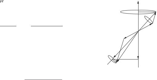
Fig. 5.11 The projection of the contributions to the total magnetic moment from the orbital motion and the spin are projected along J.
19Components perpendicular to J time-average to zero.
20This statement is justified by the projection theorem (Section 5.1), derived from the more general Wigner–Eckart theorem. The theorem shows that the expectation value of the vector operator L is proportional to that of J in the basis of eigenstates |J MJ , i.e.
J MJ |L |J MJ J MJ |J |J MJ ,
and similarly for the expectation value of S. The component along the magnetic field is found by taking the dot product with B:
J MJ |L · B |J MJ
J MJ | J · B |J MJ
J MJ | Jz |J MJ = MJ .

92 The LS-coupling scheme
Fig. 5.12 The normal Zeeman e ect on the 1s2p 1P1–1s3d 1D2 line in helium. These levels split into three and five MJ states, respectively. Both levels have S = 0 and gJ = 1 so that the allowed transitions between the states give the same pattern of three components as the classical model (in Section 1.8)—this is the historical reason why it is called the normal Zeeman effect. Spectroscopists called any other pattern an anomalous Zeeman e ect, although such patterns have a straightforward explanation in quantum mechanics and arise whenever S = 0, e.g. all atoms with one valence electron have S = 1/2. The π- and σ- components arise from ∆MJ = 0 and ∆MJ = ±1 transitions, respectively. (In this example of the normal Zeeman e ect each component corresponds to three allowed electric dipole transitions with the same frequency but they are drawn with a slight horizontal separation for clarity.)
Fig. 5.13 The anomalous Zeeman effect for the 6s6p 3P2–6s7s 3S1 transition in Hg. The lower and upper levels both have the same number of Zeeman sub-levels (or MJ states) as the levels in Fig. 5.12, but give rise to nine separate components because the levels have different values of gJ . (The 6s7s configuration happens to have higher energy than 6s6p, as shown in Fig. 5.9, but the Zeeman pattern does not depend on the relative energy of the levels.)
2
1
0
−1 −2
1
0
−1
Frequency
1
0
−1
2
1
0
−1 −2
Frequency

5.6 Summary 93
B
S
|
Fig. 5.14 The Paschen–Back e ect oc- |
|
curs in a strong external magnetic field. |
|
The spin and orbital angular momen- |
L |
tum precess independently about the |
magnetic field. The states have ener- |
|
|
gies given by EPB = µBB(ML + 2MS ). |
5.6Summary
Figure 5.15 shows the di erent layers of structure in a case where the LS-coupling scheme is a good approximation, i.e. the residual electrostatic interaction dominates the two magnetic interactions (spin–orbit and with an external magnetic field). The spin–orbit interaction splits terms into di erent J levels. The Zeeman e ect of a weak magnetic field splits the levels into states of given MJ , that are also referred to as Zeeman sub-levels.
There are various ways in which this simple picture can break down.
(a) Configuration mixing occurs if the residual electrostatic interaction
−
− −
−
|
|
|
|
Fig. 5.15 The hierarchy of atomic structure for the 3s3p configuration of an alkaline earth metal atom.

94 The LS-coupling scheme
is not small compared to the energy gap between the configurat- ions—this is common in atoms with complex electronic structure.
(b)The jj-coupling scheme is a better approximation than LS-coupling or Russell–Saunders coupling when the spin–orbit interaction is greater than the residual electrostatic interaction.
(c)The Paschen–Back e ect arises when the interaction with an external magnetic field is stronger than the spin–orbit interaction (with the internal field). This condition is di cult to achieve except for atoms with a low atomic number and hence small fine structure. Similar physics arises in the study of the Zeeman e ect on hyperfine structure where the transition between the low-field and high-field regimes occurs at values of the magnetic field that are easily accessible in experiments (see Section 6.3).
Further reading
The mathematical methods that describe the way in which angular momenta couple together form the backbone of the theory of atomic structure. In this chapter the quantum mechanical operators have been treated by analogy with classical vectors (the vector model) and the Wigner–Eckart theorem was mentioned to justify the projection theorem. Graduate-level texts give a more comprehensive discussion of the quantum theory of angular momentum, e.g. Cowan (1981), Brink and Satchler (1993) and Sobelman (1996).
Exercises
(5.1) Description of the LS-coupling scheme
Explain what is meant by the central-field approximation and show how it leads to the concept of electron configurations. Explain how perturbations arising from (a) the residual electrostatic interactions, and (b) the magnetic spin–orbit interactions, modify the structure of an isolated multielectron configuration in the LS-coupling limit.
(5.2) Fine structure in the LS-coupling scheme
Show from eqn 5.4 that the J levels of the 3P term in the 3s4p configuration have a separation given by eqn 5.8 with βLS = β4p/2 (where β4ps · l is the spin–orbit interaction of the 4p-electron).
(5.3) The LS-coupling scheme and the interval rule in calcium
Write down the ground configuration of calcium (Z = 20). The line at 610 nm in the spectrum
of neutral calcium consists of three components at relative positions 0, 106 and 158 (in units of cm−1). Identify the terms and levels involved in these transitions.
The spectrum also contains a multiplet of six lines with wavenumbers 5019, 5033, 5055, 5125, 5139 and 5177 (in units of cm−1). Identify the terms and levels involved. Draw a diagram of the relevant energy levels and the transitions between them. What further experiment could be carried out to check the assignment of quantum numbers?
(5.4) The LS-coupling scheme in zinc
The ground configuration of zinc is 4s2. The seven lowest energy levels of zinc are 0, 32 311, 32 501, 32 890, 46 745, 53 672 and 55 789 (in units of cm−1). Sketch an energy-level diagram that shows these levels with appropriate quantum numbers. What evidence do these levels provide that
|
|
|
|
|
|
|
|
|
|
Exercises for Chapter 5 95 |
|||||
|
the LS-coupling scheme describes this atom. Show |
|
|
Hund’s rules the 5D term has the lowest en- |
|||||||||||
|
the electric dipole transitions that are allowed be- |
|
|
ergy.) Specify the lowest-energy term for each |
|||||||||||
|
tween the levels. |
|
|
|
|
|
|
of the five configurations nd, nd2, nd3, nd4 |
|||||||
(5.5) |
The LS-coupling scheme |
|
|
|
|
|
|
and nd5. |
|
|
|
|
|||
|
|
|
|
|
|
|
|
|
|
|
|
||||
|
|
|
|
|
|
|
(5.7) |
Transition from LSto jj-coupling |
|||||||
|
|
|
3s3p, Mg |
3s3p, Fe14+ |
|||||||||||
|
|
|
|
|
|
|
|
|
|
|
|
||||
|
|
|
|
|
|
|
|
|
|
|
|
|
|
|
|
|
|
2.1850 |
23.386 |
|
|
|
|
|
|
|
|
|
|
|
|
|
|
|
|
|
|
|
3p4s, Si |
|
|
3p7s, Si |
|||||
|
|
2.1870 |
23.966 |
|
|
|
|
|
|
|
|||||
|
|
|
|
|
|
J |
Energy (106 m−1) |
|
J |
Energy (106 m−1) |
|||||
|
|
2.1911 |
25.378 |
|
|
|
|
|
|
|
|
|
|
|
|
|
|
|
|
|
0 |
3.968 |
|
0 |
6.154 |
|
|||||
|
|
3.5051 |
35.193 |
|
|
|
|
|
|||||||
|
|
|
|
|
|
|
|
1 |
3.976 |
|
1 |
6.160 |
|
||
|
|
|
|
|
|
|
|
||||||||
|
The |
table gives the energy levels, in units of |
2 |
3.996 |
|
2 |
6.182 |
|
|||||||
|
1 |
4.099 |
|
1 |
6.188 |
|
|||||||||
|
106 m−1 measured from the ground state, of the |
|
|
||||||||||||
|
|
|
|
|
|
|
|
|
|||||||
|
|
|
|
|
|
|
|
|
|||||||
|
3s3p configuration in neutral magnesium (Z = |
The table gives J-values and energies (in units of |
|||||||||||||
|
12) and the magnesium-like ion Fe |
14+ |
. Suggest, |
||||||||||||
|
|
|
106 m−1 measured from the ground state) of the |
||||||||||||
|
with reasons, further quantum numbers to iden- |
||||||||||||||
|
tify these levels. Calculate the ratio of the spin– |
levels in the 3p4s and 3p7s configurations of sili- |
|||||||||||||
|
con. Suggest further quantum numbers to identify |
||||||||||||||
|
orbit interaction energies in the 3s3p configura- |
||||||||||||||
|
the levels. |
|
|
|
|
||||||||||
|
tion |
of Mg and Fe14+, |
and explain your result. |
|
|
|
|
||||||||
|
Discuss the occurrence in the solar spectrum of |
Why do the two configurations have nearly the |
|||||||||||||
|
same value of EJ =2 − EJ =0 but quite di erent en- |
||||||||||||||
|
a strong line at 41.726 nm that originates from |
||||||||||||||
|
Fe14+. Would you expect a corresponding tran- |
ergy separations between the two J = 1 states? |
|||||||||||||
|
sition in neutral Mg? |
|
|
|
(5.8) |
Angular-momentum coupling schemes |
|||||||||
(5.6) |
LS-coupling for configurations with equivalent |
|
|
|
|
|
|
|
|
||||||
|
electrons |
|
|
|
|
|
|
|
|
|
|
|
|
||
|
|
|
|
|
|
|
4p5s, germanium |
|
|
5p6s, tin |
|||||
|
|
|
|
|
|
|
|
|
|
|
|
||||
|
(a) |
List the values of the magnetic quantum num- |
|
J |
Energy (106 m−1) |
|
|
J |
Energy (106 m−1) |
|
|||||
|
0 |
3.75 |
|
0 |
3.47 |
|
|||||||||
|
|
bers ml1 , ms1 , ml2 and ms2 for the two elec- |
|
|
|||||||||||
|
|
trons in an np2 configuration to show that fif- |
1 |
3.77 |
|
1 |
3.49 |
|
|||||||
|
|
teen degenerate states exist within the central- |
2 |
3.91 |
|
2 |
3.86 |
|
|||||||
|
|
field approximation. Write down the values of |
1 |
4.00 |
|
1 |
3.93 |
|
|||||||
|
|
ML = ml1 + ml2 and MS = ms1 + ms2 associ- |
|
|
|
|
|
|
|
|
|||||
|
|
ated with each of these states to show that the |
The table gives the J-values and energies (in units |
||||||||||||
|
|
only possible terms in the LS-coupling scheme |
|||||||||||||
|
|
of 106 m−1 measured from the ground state) of the |
|||||||||||||
|
|
are 1S, 3P and 1D. |
|
|
|
|
levels in the configurations 4p5s in Ge and 5p6s in |
||||||||
|
|
|
|
|
|
|
|
||||||||
|
(b) |
The 1s22s22p2 configuration of doubly-ionized |
Sn. Data for the 3p4s configuration in Si are given |
||||||||||||
|
|
oxygen has levels at relative positions 0, 113, |
in the previous exercise. |
How well does the LS- |
|||||||||||
|
|
307, 20 271 and 43 184 (in units |
of cm−1) |
coupling scheme describe the energy levels of the |
|||||||||||
|
|
above the ground state, and its spectrum con- |
np(n + 1)s configurations with n = 3, 4 and 5? |
||||||||||||
|
|
tains weak emission lines at 19 964 cm−1 and |
Give a physical reason for the observed trends in |
||||||||||||
|
|
20 158 cm−1. Identify the quantum numbers |
the energy levels. |
|
|
|
|
||||||||
|
|
for each of the levels and discuss the extent to |
One of the J = 1 levels in Ge has a Land´e g-factor |
||||||||||||
|
|
which the LS-coupling scheme describes this |
of gJ = 1.06. Which level would you expect this |
||||||||||||
|
|
multiplet. |
|
|
|
|
to be and why? |
|
|
|
|
||||
|
(c) For six d-electrons, |
in the same |
sub-shell, (5.9) |
Selection rules in the LS-coupling scheme |
|||||||||||
|
|
write a list of the values of the ms and ml |
State the selection rules that determine the config- |
||||||||||||
|
|
for the individual electrons corresponding to |
urations, terms and levels that can be connected |
||||||||||||
|
|
MS = 2 and ML = 2. Briefly discuss why this |
by an electric dipole transition in the LS-coupling |
||||||||||||
|
|
is the maximum value of MS , and why ML 2 |
approximation. Explain which rules are rigorous, |
||||||||||||
|
|
for this particular value of MS . (Hence from |
and which depend on the validity of the coupling |
||||||||||||