Atomic physics (2005)

9This is not necessarily the best way to parametrise the problem for numerical calculations but it is useful for understanding the underlying physical principles.

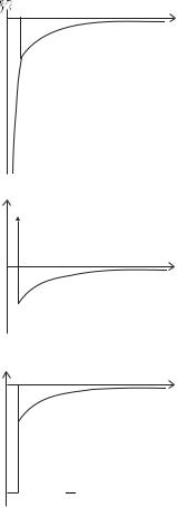
Fig. 4.4 The form of the potential energy of an electron in the central-field approximation (e2M = e2/4π 0). This approximate sketch for a sodium atom shows that the potential energy crosses

over from VCF(r) = −e2M/r at long range to −11e2M/r + Vo set; the constant Vo set comes from the integration

in eqn 4.11 (if Ze (r) = 11 for all r then

Vo set = 0 but this is not the case). For electrons with l > 0 the e ective poten-

tial should also include the term that arises from the angular momentum, as shown in Fig. 4.5.

Fig. 4.3 The change-over from the shortto the long-range is not calculated but is drawn to be a reasonable guess, using the following criteria. The typical radius of the 1s wavefunction around the nucleus of charge +Ze = +11e is about a0/11, and so Ze will start to drop at this distance. We know that Ze 1 at the distance at which the 3d wavefunction has appreciable probability since that eigenstate has nearly the same energy as in hydrogen. The form of the function Ze (r) can be found quantitatively by the Thomas–Fermi method described in Woodgate (1980).

At large distances the other N − 1 electrons screen most of the nuclear charge so that the field is equivalent to that of charge +1e:

and Ze (r) → 1 as r → ∞, as sketched in Fig. 4.3.9 The potential energy of an electron in the central field is obtained by integrating from

The form of this potential is shown in Fig. 4.4.

So far, in our discussion of the sodium atom in terms of the wavefunction of the valence electron in a central field we have neglected

the fact that the central field itself depends on the configuration of the electrons in the atom. For a more accurate description we must take into account the e ect of the outer electron on the other electrons, and hence on the central field. The energy of the whole atom is the sum of the energies of the individual electrons (in eqn 4.6), e.g. a sodium atom in the 3s configuration has energy E 1s22s22p6 3s = 2E1s +2E2s +6E2p + E3s = Ecore + E3s. This is the energy of the neutral atom relative to the bare nucleus (Na11+).10 It is more useful to measure the binding energy relative to the singly-charged ion (Na+) with energy E 1s22s22p6 =

2E1s +2E2s+6E2p = Ecore. The dashes are significant—the ten electrons in the ion and the ten electrons in the core of the atom have slightly

di erent binding energies because the central field is not the same in the two cases. The ionization energy is IE = Eatom − Eion = (Ecore − Ecore) + E3s. From the viewpoint of valence electrons, the di erence in Ecore between the neutral atom and the ion can be attributed to core polarization, i.e. a change in the distribution of charge in the core produced by the valence electron.11 To calculate the energy of multi-

10This is a crude approximation, especially for inner electrons.

11This e ect is small in the alkalis and it is reasonable to use the frozen core

approximation that assumes Ecore Ecore. This approximation becomes more accurate for a valence electron in higher levels where the influence on the core becomes smaller.

68 The alkalis

12This is in contrast to an infinite square well where confinement to a region of fixed dimensions gives energies proportional to n2, where n is an integer.

electron atoms properly we should consider the energy of the whole system rather than focusing attention on only the valence electron. For example, neon has the ground configuration 1s22s22p6 and the electric field changes significantly when an electron is excited out of the 2p subshell, e.g. into the 1s22s22p53s configuration.

Quantum defects can be considered simply as empirical quantities that happen to give a good way of parametrising the energies of the alkalis but there is a physical reason for the form of eqn 4.1. In any potential that tends to 1/r at long range the levels of bound states bunch together as the energy increases—at the top of the well the classically allowed region gets larger and so the intervals between the eigenenergies and the stationary solutions get smaller.12 More quantitatively, in Exercise 1.12 it was shown, using the correspondence principle, that such a potential has energies E 1/k2, with ∆k = 1 between energy levels, but k is not itself necessarily an integer. For the special case of a potential proportional to 1/r for all distances, k is an integer that we call the principal quantum number n and the lowest energy level turns out to be n = 1. For a general potential in the central-field approximation we have seen that it is convenient to write k in terms of the integer n as k = n −δ, where δ is a non-integer (quantum defect). To find the actual energy levels of an alkali and hence δ (for a given value of l) requires the numerical calculation of the wavefunctions, as outlined in the following section.

4.4Numerical solution of the Schr¨odinger equation

Before describing particular methods of solution, let us look at the general features of the wavefunction for particles in potential wells. The radial equation for P (r) has the form

where the potential V (r) includes the angular momentum term in eqn 4.7. Classically, the particle is confined to the region where E −V (r) > 0 since the kinetic energy must be positive. The positions where E = V (r) are the classical turning points where the particle instantaneously comes to rest, cf. at the ends of the swing of a pendulum. The quantum wavefunctions are oscillatory in the classically allowed region, with the curvature and number of nodes both increasing as E − V (r) increases, as shown in Fig. 4.6. The wavefunctions penetrate some way into the classically forbidden region where E − V (r) < 0; but in this region the solutions decay exponentially and the probability falls o rapidly.

How can we find P (r) in eqn 4.12 without knowing the potential V (r)? The answer is firstly to find the wavefunctions for a potential VCF(r) that is ‘a reasonable guess’, consistent with eqn 4.11 and the limits on the central electric field in the previous equations. Then, secondly, we

make the assumed potential correspond closely to the real potential, as described in the next section. Equation 4.12 is a second-order di erential equation and we can numerically calculate P (r), the value of the function at r, from two nearby values, e.g. u (r − δr) and u (r − 2δr).13 Thus, working from near r = 0, the method gives the numerical value of the function at all points going out as far as is necessary. The region of the calculation needs to extend beyond the classical turning point(s) by an amount that depends on the energy of the wavefunction being calculated. These general features are clearly seen in the plots produced in Exercise 4.10. Actually, that exercise describes a method of finding the radial wavefunction R(r) rather than P (r) = rR (r) but similar principles apply.14 If you carry out the exercise you will find that the behaviour at large r depends very sensitively on the energy E—the wavefunction diverges if E is not an eigenenergy of the potential—this gives a way of searching for those eigenenergies. If the wavefunction diverges upwards for E and downwards for E then we know that an eigenenergy of the system Ek lies between these two values, E < Ek < E . Testing further values between these upper and lower bounds narrows the range and gives a more precise value of Ek (as in the Newton–Raphson method for finding roots). This so-called ‘shooting’ method is the least sophisticated method of computing wavefunctions and energies, but it is adequate for illustrating the principles of such calculations. Results are not given here since they can readily be calculated—the reader is strongly encouraged to implement the numerical method of solution, using a spreadsheet program, as described in Exercise 4.10. This shows how to find the wavefunctions for an electron in an arbitrary potential and verifies that the energy levels obey a quantum defect formula such as eqn 4.1 in any potential that is proportional to 1/r at long range (see Fig. 4.7).

13The step size δr must be small compared to the distance over which the wavefunction varies; but the number of steps must not be so large that round- o errors begin to dominate.

14In a numerical method there is no reason why we should not calculate the wavefunction directly; P (r) was introduced to make the equations neater in the analytical approach.

70 The alkalis

Fig. 4.7 Simple modifications of the potential energy that could be used for the numerical solution of the Schr¨odinger equation described in Ex-

ercise 4.10. For all these potentials V (r) = −e2/4π 0r for r rcore. (a) Inside the radial distance rcore the potential energy is V (r) = −Ze2/4π 0r +

Vo set, drawn here for Z = 3 and an o set chosen so that V (r) is continuous

at r = rcore. This corresponds to the situation where the charge of the core is an infinitely thin shell. The deep potential in the inner region means that the wavefunction has a high curvature, so small steps must be used in the numerical calculation (in this region). The hypothetical potentials in (b) and (c) are useful for testing the numerical method and for showing why the eigenenergies of any potential proportional to 1/r at long range obey a quantum defect formula (like eqn 4.1). The form of the solution depends sensitively on the energy in the outer region r rcore, but in the inner region where |E| |V (r)| it does not, e.g. the number of nodes (‘wiggles’) in this region changes slowly with energy E. Thus, broadly speaking, the problem reduces to finding the wavefunction in the outer region that matches boundary conditions, at r = rcore, that are almost independent of the energy—the potential energy curve shown in (b) is an extreme example that gives useful insight into the behaviour of the wavefunction for more realistic central fields.

(a)

(b)

0

(c)

0

4.4.1Self-consistent solutions

The numerical method described above, or a more sophisticated one, can be used to find the wavefunctions and energies for a given potential in the central-field approximation. Now we shall think about how to determine VCF itself. The potential of the central field in eqn 4.2 includes the electrostatic repulsion of the electrons. To calculate this mutual repulsion we need to know where the electrons are, i.e. their wavefunctions, but to find the wavefunctions we need to know the potential. This argument is circular. However, going round and round this loop can be useful in the following sense. As stated above, the method starts by making a reasonable estimate of VCF and then computing the electronic wavefunctions for this potential. These wavefunctions are then used to calculate a new average potential (using the central-field approximation) that is more realistic than the initial guess. This improved potential is then used to calculate more accurate wavefunctions, and so on. On suc-

cessive iterations, the changes in the potential and wavefunctions should get smaller and converge to a self-consistent solution, i.e. where the wavefunctions give a certain VCF(r), and solving the radial equation for that central potential gives back the same wavefunctions (within the required precision).15 This self-consistent method was devised by Hartree. However, the wavefunctions of multi-electron atoms are not simply products of individual wavefunctions as in eqn 4.5. In our treatment of the excited configurations of helium we found that the two-electron wavefunctions had to be antisymmetric with respect to the permutation of the electron labels. This symmetry requirement for identical fermions was met by constructing symmetrised wavefunctions that were linear combinations of the simple product states (i.e. the spatial part of these functions is

15The number of iterations required, before the changes when going round the loop become very small, depends on how well the initial potential is chosen, but the final self-consistent solution should not depend on the initial choice. In general, it is better to let a computer do the work rather than expend a lot of e ort improving the starting point.

17The wavefunction for an alkali metal atom in the central-field approximation is a product of a radial wavefunction (which does not have an analytical expression) and angular momentum eigenfunctions (as in hydrogen).

ψspin = |ms = +1/2 or |ms = −1/2 .

19Proof of these commutation relations: [sxlx + sy ly + sz lz , lz ] = sx [lx, lz ] +sy [ly , lz ] = −isxly +isy lx = 0. Similarly, [sxlx + sy ly + sz lz , sz ] =

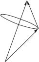
j s

l

Fig. 4.8 The total angular momentum of the atom j = l + s is a fixed quantity in the absence of an external torque. Thus an interaction between the spin and orbital angular momenta βs · l causes these vectors to rotate (precess) around the direction of j as shown.

20As for helium in Section 3.2 and in the classical treatment of the normal Zeeman e ect in Section 1.8.

21These commutation relations for the operators correspond to the conservation of the total angular momentum, and its component along the z-axis. Only an external torque on the atom a ects these quantities. The spin–orbit interaction is an internal interaction.

(a)The possible values of the total angular momentum obtained by the addition of the electron’s spin, s = 1/2, and its orbital angular momentum are j = l + 1/2 or l − 1/2. This is a consequence of the rules for the addition of angular momentum in quantum mechanics (vector addition but with the resultant quantised).

(b)The vectors have squared magnitudes given by j2 = j(j + 1), l2 = l(l + 1) and s2 = 3/4, where j and l are the relevant angular momentum quantum numbers.

Step (b) arises from taking the expectation values of the quantum operators in the Hamiltonian for the spin–orbit interaction. This is not straightforward since the atomic wavefunctions R(r) |l ml s ms are not eigenstates of this operator17—this means that we must face the complications of degenerate perturbation theory. This situation arises frequently in atomic physics and merits a careful discussion.

We wish to determine the e ect of an interaction of the form s · l on the angular eigenfunctions |l ml s ms . These are eigenstates of the operators l2, lz , s2 and sz labelled by the respective eigenvalues.18 There

are 2(2l +1) degenerate eigenstates for each value of l because the energy does not depend on the orientation of the atom in space, or the direction of its spin, i.e. energy is independent of ml and ms. The states |l ml s ms are not eigenstates of s · l because this operator does not commute with lz and sz : [s · l, lz ] = 0 and [s · l, sz ] = 0.19 Quantum operators only have simultaneous eigenfunctions if they commute. Since |l ml s ms is

in fine structure. Good quantum numbers correspond to constants of motion in classical mechanics—the magnitudes of l and s are constant but the orientations of these vectors change because of their mutual interaction, as shown in Fig. 4.8. If we try to evaluate the expectation value using wavefunctions that are not eigenstates of the operator then things get complicated. We would find that the wavefunctions are mixed by the perturbation, i.e. in the matrix formulation of quantum mechanics the matrix representing the spin–orbit interaction in this basis has o - diagonal elements. The matrix could be diagonalised by following the standard procedure for finding the eigenvalues and eigenvectors,20 but a p-electron gives six degenerate states so the direct approach would require the diagonalisation of a 6×6 matrix. It is much better to find the eigenfunctions at the outset and work in the appropriate eigenbasis. This ‘look-before-you-leap’ approach requires some preliminary reasoning.

We define the operator for the total angular momentum as j = l + s.

The operator j2 commutes with the interaction, as does its component jz : !s · l, j2" = 0 and [s · l, jz ] = 0. Thus j and mj are good quantum

numbers.21 Hence suitable eigenstates for calculating the expectation value of s · l are |l s j mj . Mathematically these new eigenfunctions can be expressed as combinations of the old basis set:

Each eigenfunction labelled by l, s, j and mj is a linear combination of the eigenfunctions with the same values of l and s but various values of ml and ms. The coe cients C are the Clebsch–Gordan coe cients and their values for many possible combinations of angular momenta are tabulated in more advanced books. Particular values of Clebsch– Gordan coe cients are not needed for the problems in this book but it is important to know that, in principle, one set of functions can be expressed in terms of another complete set—with the same number of eigenfunctions in each basis.

Finally, we use the identity22 j2 = l2 + s2 + 2s · l to express the expectation value of the spin–orbit interaction as

lsjmj | s · l |lsjmj = 12 lsjmj | j2 − l2 − s2 |lsjmj

= 12 {j(j + 1) − l (l + 1) − s (s + 1)} .

The states |lsjmj are eigenstates of the operators j2, l2 and s2. The importance of the proper quantum treatment may not yet be apparent since all we appear to have gained over the vector model is being able to write the wavefunctions symbolically as |lsjmj . We will, however, need the proper quantum treatment when we consider further interactions that perturb these wavefunctions.

22This applies both for vector operators, where j2 = jx2 + jy 2 + jz 2, and

for classical vectors where this is simply j2 = |j|2.

4.6Fine structure in the alkalis

The fine structure in the alkalis is well approximated by an empirical modification of eqn 2.56 called the Land´e formula:

In the denominator the e ective principal quantum number cubed (n )3 (defined in Section 4.2) replaces n3. The e ective atomic number Ze , which was defined in the discussion of the central-field approximation, tends to the inner atomic number Zi Z as r → 0 (where the electron ‘sees’ most of the nuclear charge); outside the core the field corresponds to an outer atomic number Zo 1 (for neutral atoms). The Land´e formula can be justified by seeing how the central-field approximation modifies the calculation of the fine structure in hydrogen (Section 2.3.2). The spin–orbit interaction depends on the electric field that the electron moves through; in an alkali metal atom this field is proportional to Ze (r)r/r3 rather than r/r3 as in hydrogen.23 Thus the expectation value of the spin–orbit interaction depends on

23This modification is equivalent to using VCF in place of the hydrogenic potential proportional to 1/r.

74 The alkalis

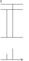
Frequency

Fig. 4.9 The fine-structure components of a p to s transition, e.g. the

3 S1/2–3 P1/2 and 3 S1/2–3 P3/2 transitions in sodium. (Not to scale.) The

statistical weights of the upper levels lead to a 1:2 intensity ratio.

24The rates of the allowed transitions depend on integrals involving the radial wavefunctions (carried out numerically for the alkalis) and the integrals over the angular part of the wavefunction given in Section 2.2.1, where we derived the selection rules.

25This shortened form of the full LS- coupling scheme notation gives all the necessary information for a single electron, cf. 3s 2S1/2–3p 2P3/2.

26This must be true for the physical reason that the decay rate is the same whatever the spatial orientation of the atom, and similarly for the spin states. All the di erent angular states have the same radial integral, i.e. that between the 3p and 3s radial wavefunctions.

27This normal situation for fine structure may be modified slightly in a case like caesium where the large separation of the components means that the frequency dependence of the lifetime (eqn 1.24) leads to di erences, even though the matrix elements are similar.

rather than 1/r3 as in hydrogen (eqn 2.51). This results in fine structure for the alkalis, given by the Land´e formula, that scales as Z2—this lies between the dependence on Z4 for hydrogenic ions (no screening) and the other extreme of no dependence on atomic number for complete screening. The e ective principal quantum number n is remarkably similar across the alkalis, as noted in Section 4.2.

As a particular numerical example of the scaling, consider the fine structure of sodium (Z = 11) and of caesium (Z = 55). The 3p configuration of sodium has a fine-structure splitting of 1700 m−1, so for a Z2-dependence the fine structure of the 6p configuration of caesium should be (using n from Table 4.2)

logarithmic plot of the energies of the gross and fine structure against atomic number is given in Fig. 5.7. This shows that the actual trend of the fine structure lies close to the Z2-dependence predicted.)

The fine structure causes the familiar yellow line in sodium to be a doublet comprised of the two wavelengths λ = 589.0 nm and 589.6 nm. This, and other doublets in the emission spectrum of sodium, can be resolved by a standard spectrograph. In caesium the transitions between the lowest energy configurations (6s–6p) give spectral lines at λ = 852 nm and 894 nm—this ‘fine structure’ is not very fine.

4.6.1Relative intensities of fine-structure transitions

The transitions between the fine-structure levels of the alkalis obey the same selection rules as in hydrogen since the angular momentum functions are the same in both cases. It takes a considerable amount of calculation to find absolute values of the transition rates24 but we can find the relative intensities of the transitions between di erent fine-structure levels from a simple physical argument. As an example we shall look at p to s transitions in sodium, as shown in Fig. 4.9. The 3 S1/2–3 P1/2 transition has half the intensity of the 3 S1/2–3 P3/2 transition.25 This 1:2 intensity ratio arises because the strength of each component is proportional to the statistical weight of the levels (2j + 1). This gives 2:4 for j = 1/2 and 3/2. To explain this we first consider the situation without fine structure. For the 3p configuration the wavefunctions have the form R3p(r) |lmlsms and the decay rate of these states (to 3s) is independent of the values of ml and ms.26 Linear combinations of the states R(r) |lmlsms with di erent values of ml and ms (but the same values of n, l and s, and hence the same lifetime) make up the eigenstates of the fine structure, |lsjmj . Therefore an alkali atom has the same lifetime for both values of j.27

If each state has the same excitation rate, as in a gas discharge lamp for example, then all the states will have equal populations and the intensity of a given component of the line is proportional to the number of contributing mj states. Similarly, the fine structure of transitions from s to p configurations, e.g. 3 P3/2–5 S1/2 and 3 P1/2–5 S1/2, have an intensity ratio of 2:1—in this case the lower frequency component has twice the intensity of the higher component, i.e. the opposite of the p to s transition shown in Fig. 4.9 (and such information can be used to identify the lines in an observed spectrum). More generally, there is a sum rule for intensities: the sum of the intensities to, or from, a given level is proportional to its degeneracy; this can be used when both upper and lower configurations have fine structure (see Exercise 4.8).

The discussion of the fine structure has shown that spin leads to a splitting of energy levels of a given n, of which l levels have di erent j. These fine-structure levels are degenerate with respect to mj , but an external magnetic field removes this degeneracy. The calculation of the e ect of an external magnetic field in Chapter 1 was a classical treatment that led to the normal Zeeman e ect. This does not accurately describe what happens for atoms with one valence electron because the contribution of the spin magnetic moment leads to an anomalous Zeeman e ect. The splitting of the fine-structure level into 2j + 1 states (or Zeeman sub-levels) in an applied field is shown in Fig. 4.10. It is straightforward to calculate the Zeeman energy for an atom with a single valence electron, as shown in quantum texts, but to avoid repetition the standard treatment is not given here; in the next chapter we shall derive a general formula for the Zeeman e ect on atoms with any number of valence electrons that covers the single-electron case (see Exercise 5.13). We also look at the Zeeman e ect on hyperfine structure in Chapter 6.

4.6Fine structure in the alkalis 75

Energy

0

Fig. 4.10 In an applied magnetic field of magnitude B the four states of di erent mj of the 2P3/2 level have energies of EZeeman = gj µBBmj —the factor gj arises from the projection of the contributions to the magnetic moment from l and s onto j (see Exercise 5.13).