

Atomic physics (2005)
.pdf126The interaction of atoms with radiation
7.2The Einstein B coe cients
In the previous section we found the e ect of an electric field E0 cos (ωt) on the atom. To relate this to Einstein’s treatment of the interaction with broadband radiation we consider what happens with radiation of energy density ρ (ω) in the frequency interval ω to ω +dω. This produces an electric field of amplitude E0 (ω) given by ρ (ω) dω = 0E02 (ω) /2. For this narrow (almost monochromatic) slice of the broad distribution eqn 7.12 gives
|
|
|
|
E (ω) |
|
2 |
|
2 X 2 |
|
2ρ (ω) dω |
|
||
|Ω|2 |
= |
eX12 |
|
0 |
|
|
= e | 212| |
0 . |
(7.17) |
||||
|
|
|
|
|
|
|
|
|
|
|
|
|
|
|
|
|
|
|
|
|
|
|
|
|
|
|
|
6As in optics experiments with broadband light, it is intensities that are summed, e.g. the formation of whitelight fringes in the Michelson interferometer.
Integration of eqn 7.15 over frequency gives the excitation probability for the broadband radiation as
c |
(t) |
2 |
= |
2e2 |X12|2 |
ω0 +∆/2 |
ρ (ω) |
sin2 {(ω0 − ω)t/2} |
dω . (7.18) |
|
| |
ω0−∆/2 |
||||||||
| 2 |
|
|
0 2 |
|
(ω0 − ω)2 |
||||
We integrate the squares of the amplitudes, rather than taking the square of the total amplitude, since contributions at di erent frequencies do not interfere.6 The range of integration ∆ must be large compared to the extent of the sinc function, but this is easily fulfilled since as time increases this function becomes sharply peaked at ω0. (In the limit t → ∞ it becomes a Dirac delta function—see Loudon (2000).) Over
the small range about ω0 where the sinc function has an appreciable value, a smooth function like ρ (ω) varies little, so we take ρ (ω0) outside the integral. A change of variable to x = (ω − ω0) t/2, as in eqn 7.16, leads to
|
2e2 X12 |
2 |
|
t |
+φ sin2 x |
|
|
|
|c2 (t)|2 |
| |
| |
ρ (ω0) × |
|
−φ |
|
dx . |
(7.19) |
0 2 |
|
2 |
x2 |
|||||
The integration has limits of x = ±φ = ±∆t/4 π and the integral approximates closely to −∞∞ x−2 sin2 x dx = π. We make this assumption of a long interaction to find the steady-state excitation rate for broadband radiation. The probability of transition from level 1 to 2 increases linearly with time corresponding to a transition rate of
R12 = |
|c2 (t)|2 |
= |
πe2 |X12|2 |
ρ (ω0) . |
(7.20) |
|
t |
0 2 |
|||||
|
|
|
|
Comparison with the upward rate B12ρ (ω) in Einstein’s treatment of radiation (eqn 1.25) shows that
B12 = |
πe2 |D12|2 |
, |
(7.21) |
|
3 0 2 |
||||
|
|
|
where |X12|2 → |D12|2 /3, and D12 is the magnitude of the vector
D |
= 1 |
| |
r 2 |
ψ r ψ |
2 |
d3r . |
(7.22) |
12 |
|
| ≡ |
1 |
|
|
7.3 Interaction with monochromatic radiation 127
The factor of 1/3 arises from averaging of D · erad, where erad is a unit vector along the electric field, over all the possible spatial orientations of the atom (see Exercise 7.6). The relation between A21 and B12 in eqn 1.32 leads to
A21 = |
g1 |
|
4α |
× ω3 |D12|2 , |
(7.23) |
g2 |
|
3c2 |
where α = e2/ (4π 0 c) is the fine-structure constant. The matrix element between the initial and final states in eqn 7.22 depends on an integral involving the electronic wavefunctions of the atom so, as emphasised previously, the Einstein coe cients are properties of the atom. For a typical allowed transition the matrix element has an approximate value of D12 3a0 (this can be calculated analytically for hydrogenic systems). Using this estimate of D12 in the equation gives A21 2π × 107 s−1 for a transition of wavelength λ = 6 × 10⁻⁷ m and g1 = g2 = 1. Although we have not given a physical explanation of spontaneous emission, Einstein’s argument allows us to calculate its rate; he obtained the relation between A21 and B21 and we have used TDPT to determine B21 from the atomic wavefunctions. For a two-level atom with an allowed transition between the levels the quantum mechanical result corresponds closely to the treatment of radiative decay using classical electromagnetism in Section 1.6.
7.3Interaction with monochromatic radiation
The derivation of eqns 7.14 assumed that the monochromatic radiation perturbed the atom only weakly so that most of the population stayed in the initial state. We shall now find a solution without assuming a weak field. We write eqn 7.9 as
. |
= c2 |
(ei(ω−ω0)t + e−i(ω+ω0)t) |
Ω |
|
(7.24) |
|
ic1 |
|
|
, |
|||
2 |
|
|||||
and similarly for eqn 7.10. The term with (ω + ω0) t oscillates very fast and therefore averages to zero over any reasonable interaction time—this is the rotating-wave approximation (Section 7.1.2) and it leads to
. |
= c2ei(ω−ω0)t |
Ω |
|
|
|
|
|
|
|||||
|
|
ic1 |
|
, |
|
|
|
|
|
|
|||
2 |
|
|
|
|
|
(7.25) |
|||||||
. |
|
|
|
|
Ω |
|
|
||||||
|
|
|
|
|
|
|
|||||||
|
|
ic2 |
= c1e−i(ω−ω0)t |
|
|
. |
|
|
|||||
2 |
|
|
|||||||||||
These combine to give |
|
|
|
|
|
|
|
|
|
|
|
||
|
d2c |
|
dc |
|
Ω |
|
2 |
c2 = 0 . |
(7.26) |
||||
|
dt22 + i (ω − ω0) dt2 + |
2 |
|
|
|||||||||
|
|
|
|
|
|
|
|
|
|
|
|
|
|
|
|
|
|
|
|
|
|
|
|
|
|
|
|
The solution of this second-order di erential |
equation |
for the initial con- |
|||||||||||
ditions c1 (0) = 1 and c2 (0) = 0 gives the probability of being in the upper state as7
7For transitions between bound states the frequency Ω is real, so |Ω|2 = Ω2.
128 The interaction of atoms with radiation |
|
|
|
|
|
|
|c2 (t)|2 = |
Ω2 |
|
W t |
, |
|
|
|
sin2 |
|
(7.27) |
|||
W 2 |
2 |
|||||
where |
|
|
|
|
|
|
W 2 = Ω2 + (ω − ω0)2 . |
(7.28) |
|||||
8This is partly a consequence of the dependence on ω3 in eqn 7.23, but also because the magnetic dipole transitions have smaller matrix elements than electric dipole transitions. For electric dipole transitions in the optical region spontaneous emission washes out the Rabi oscillations on a time-scale of tens of nanoseconds (τ = 1/A21, assuming that the predominant decay is from 2 to 1, and we estimated A12 above). Nevertheless, experimenters have observed coherent oscillations by driving the transition with intense laser radiation to give a high Rabi frequency (Ωτ > 1).
At resonance ω = ω0 and W = Ω, so |
|
|
|
|
|c2 (t)|2 = sin2 |
|
Ωt |
. |
(7.29) |
|
||||
2 |
The population oscillates between the two levels. When Ωt = π all the population has gone from level 1 into the upper state, |c2 (t)|2 = 1, and when Ωt = 2π the atom has returned to the lower state. This behaviour is completely di erent from that of a two-level system governed by rate equations where the populations tend to become equal as the excitation rate increases and population inversion cannot occur. These Rabi oscillations between the two levels are readily observed in radio-frequency spectroscopy, e.g. for transitions between Zeeman or hyperfine states. Radio-frequency and microwave transitions have negligible spontaneous emission so that, in most cases, the atoms evolve coherently.8
9This can be shown by solving eqns 7.25 (and 7.26) for ω = ω0.
7.3.1The concepts of π-pulses and π/2-pulses
A pulse of resonant radiation that has a duration of tπ = π/Ω is called a π-pulse and from eqn 7.29 we see that Ωt = π results in the complete transfer of population from one state to the other, e.g. an atom initially in |1 ends up in |2 after the pulse. This contrasts with illumination by broadband radiation where the populations (per state) become equal as the energy density ρ (ω) increases. More precisely, a π-pulse swaps the states in a superposition:9
c1 |1 + c2 |2 → −i {c1 |2 + c2 |1 } . |
(7.30) |
This swap operation is sometimes also expressed as |1 ↔ |2 , but the factor of −i is important in atom interferometry, as shown in Exercise 7.3.
Interferometry experiments also use π/2-pulses that have half the duration of a π-pulse (for the same Rabi frequency Ω). For an atom initially in state |1 , the π/2-pulse puts its wavefunction into a superposition of states |1 and |2 with equal amplitudes (see Exercise 7.3).
7.3.2The Bloch vector and Bloch sphere
In this section we find the electric dipole moment induced on a atom by radiation, and introduce a very powerful way of describing the behaviour of two-level systems by the Bloch vector. We assume that the electric field is along ex, as in eqn 7.12. The component of the dipole along this
direction is given by the expectation value
−eDx(t) = − Ψ†(t) ex Ψ(t) d3r . |
(7.31) |
7.3 Interaction with monochromatic radiation 129
Using eqn 7.5 for Ψ (t) gives this dipole moment of the atom as |
|
|||||
Dx(t) = |
|
|
iω0t |
iω0t |
|
|
|
c1e−iω1tψ1 + c2e−iω2tψ2 x c1e−iω1tψ1 + c2e−iω2tψ2 d3r |
|||||
= c2c1X21e |
|
+ c1c2X12e− . |
(7.32) |
|||
Here ω0 = ω2 − ω1. The dipole moment is a real quantity since from eqn 7.13 we see that X21 = (X12) , and also X11 = X22 = 0. To calculate this dipole moment induced by the applied field we need to know the bilinear quantities c1c2 and c2c1. These are some of the elements of the density matrix10
|
|
|
|
|
|
|
1 |
| |
|
| |
|
2 |
|
|
|
|
|
c1 |
|
|
|
|
c |
2 |
c |
c |
|
ρ11 |
ρ12 |
|
|||
|Ψ Ψ| = |
c2 |
c1 |
c2 |
|
= |
1|c2c| |
c2 |
|
2 |
= |
ρ21 |
ρ22 |
. (7.33) |
|||
O -diagonal elements of the density matrix are called coherences and they represent the response of the system at the driving frequency (eqn 7.32). The diagonal elements |c1|2 and |c2|2 are the populations. We define the new variables
c1 |
= c1e−iδt/2 , |
(7.34) |
||
%2 |
= c |
2 |
eiδt/2 , |
(7.35) |
c |
|
|||
% |
|
|
|
|
where δ = ω − ω0 is the detuning of the radiation from the atomic resonance. This transformation does not a ect the populations ( ρ%11 = ρ11 and ρ%22 = ρ22) but the coherences become ρ%12 = ρ12 exp(−iδt) and ρ%21 = ρ21 exp(iδt) = (ρ%12) . In terms of these coherences the dipole moment is11
= −eX12 |
|
|
− |
|
|
% |
% |
|
|
−eDx (t) = −eX12 |
|
ρ12eiω0t + ρ21e−iω0t |
|
= −eX12 ρ12eiωt + ρ21e−iωt |
|
||||
|
(u cos ωt |
|
v sin ωt) . |
|
|
|
(7.36) |
||
The coherences ρ%12 and ρ%21 give the response of the atom at ω, the (angular) frequency of the applied field. The real and imaginary parts of ρ%12 (multiplied by 2) are:
10This is the outer product of |Ψ and
its Hermitian conjugate Ψ| ≡ |Ψ †, the transposed conjugate of the matrix representing |Ψ . This way of writing the information about the two levels is an extremely useful formalism for treating quantum systems. However, we have no need to digress into the theory of density matrices here and we simply adopt it as a convenient notation.
11We assume that X12 is real. This is true for transitions between two bound states of the atom—the radial wavefunctions are real and the discussion of selection rules shows that the integration over the angular momentum eigenfunctions also gives a real contribution to the matrix element—the integral over φ is zero unless the terms containing powers of exp(−iφ) cancel.
u = ρ%12 + ρ%21 ,
(7.37)
v = −i (ρ%12 − ρ%21) .
In eqn 7.36 we see that u and v are the in-phase and quadrature components of the dipole in a frame rotating at ω. To find expressions for ρ%12, ρ%21 and ρ22, and hence u and v, we start by writing eqns 7.25 for c1 and c2 in terms of δ as follows:12
. |
|
iδt Ω |
(7.38) |
||||
ic1 |
= c2e |
|
|
|
, |
|
|
2 |
|
||||||
. |
|
|
|
Ω |
|
||
ic2 |
= c1e−iδt |
|
. |
(7.39) |
|||
2 |
|||||||
Di erentiation of eqn 7.34 yields13
12All the steps in this lengthy procedure cannot be written down here but enough information is given for meticulous readers to fill in the gaps.
13Spontaneous decay is ignored here— this section deals only with coherent evolution of the states.
130 The interaction of atoms with radiation
14This is appropriate for calculating absorption. Alternatively, ρ22 − ρ11 could be chosen as a variable—this population inversion determines the gain in lasers.
|
|
|
|
. |
|
. |
|
|
|
|
|
|
|
|
|
|
|
|
|
iδ |
|
|
|
|
|
|
|
|
|
|
|
|
|
|
|
|
c1 = c1e−iδt/2 − |
|
c1e−iδt/2 . |
|
|
|
|
(7.40) |
|||||||||||||||||||||
|
|
|
|
2 |
|
|
|
|
||||||||||||||||||||||||
Multiplication. by i |
and the use of eqns 7.38, 7.34 and 7.35 yields an |
|||||||||||||||||||||||||||||||
|
% |
|
|
|
|
|
|
|
|
|
|
|
|
|
|
|
|
|
|
|
. |
|
|
|
|
|
|
|
|
|||
equation for c1 (and similarly we can obtain c2 from eqn 7.39): |
||||||||||||||||||||||||||||||||
|
|
|
|
|
|
. |
|
|
|
|
2 |
|
|
|
|
%1 |
− |
%2 |
|
|
|
|
|
|
|
|
|
|||||
|
|
|
|
|
|
i%2 |
|
|
|
|
|
|
|
|
|
|
|
|
|
|
|
|
||||||||||
% |
|
|
|
|
ic1 |
= |
|
|
1 |
|
(δ c1 |
+ Ω c2)%, |
|
|
|
|
|
|
|
|||||||||||||
|
|
|
2 |
|
|
|
|
|
|
|
(7.41) |
|||||||||||||||||||||
|
|
|
|
|
|
. |
|
|
|
|
|
|
1 |
|
|
|
|
|
|
|
|
|
|
|
|
|
|
|
|
|
||
|
|
|
|
|
|
|
= |
|
(Ω c |
|
|
|
|
) . |
|
|
|
|
|
|
|
|||||||||||
|
|
|
|
|
|
c |
|
|
|
|
δ c |
|
|
|
|
|
|
|
||||||||||||||
|
|
|
|
|
|
|
|
|
|
|
|
|
|
|
|
|
|
|||||||||||||||
From these we find that the% |
|
|
|
|
|
|
|
|
|
|
|
|
|
|
|
|
. |
|
= c |
|
. |
. |
|
c , etc. are |
||||||||
|
time derivatives% % ρ |
12 |
1 |
c + c |
1 |
|||||||||||||||||||||||||||
|
|
|
|
|
|
|
|
|
|
|
|
|
|
|
|
|
|
|
|
|
|
|
|
|
|
|
2 |
|
2 |
|||
|
dρ12 |
= |
|
dρ21 |
|
|
|
|
= |
|
|
|
iδ ρ12 |
+ |
iΩ |
(ρ |
|
|
ρ |
) , |
|
|
||||||||||
|
|
|
|
|
|
|
|
|
|
|
|
|
|
|
|
|
|
|
||||||||||||||
|
|
|
|
dt |
|
|
− |
|
% |
11 % %22 |
% % |
|||||||||||||||||||||
|
dt |
|
|
|
|
|
|
|
|
|
|
|
|
2 |
|
|
− |
|
|
|
(7.42) |
|||||||||||
|
ρ |
|
|
dρ |
|
|
|
|
|
iΩ |
|
|
|
|
|
|
|
|
|
|
|
|
|
|
|
|||||||
|
d%22 |
= |
|
%11 |
|
= |
|
|
(ρ21% |
|
ρ12) . |
|
|
|
|
|
|
|
||||||||||||||
|
|
− dt |
|
|
|
|
|
|
|
|
|
|
|
|||||||||||||||||||
|
dt |
|
|
|
|
|
2 |
|
|
|
|
− |
|
|
|
|
|
|
|
|
|
|
|
|||||||||
|
|
|
|
|
|
|
|
|
|
|
|
|
|
|
|
|
|
|
normalisation in eqn 7.7, i.e. |
|||||||||||||
The last equation is consistent with% |
|
|
% |
|
|
|
|
|
|
|
|
|
|
|||||||||||||||||||
|
|
|
|
|
|
|
|
ρ22 + ρ11 = 1 . |
|
|
|
|
|
|
|
|
(7.43) |
|||||||||||||||
In terms of u and v in eqns 7.37 these equations become |
|
|
|
|||||||||||||||||||||||||||||
|
|
|
|
. |
|
|
|
|
|
|
|
|
|
|
|
|
|
|
|
|
|
|
|
|
|
|
|
|
|
|
|
|
|
|
|
|
|
u = δ v , |
|
|
|
|
|
|
|
|
|
|
|
|
|
|
|
|
|
||||||||||
|
|
|
|
. |
|
|
−δ u + Ω (ρ11 − ρ22) , |
|
|
|
|
|
||||||||||||||||||||
|
|
|
|
|
v = |
|
|
|
|
|
(7.44) |
|||||||||||||||||||||
|
|
|
|
. |
|
= |
|
|
Ωv |
|
|
|
|
|
|
|
|
|
|
|
|
|
|
|
|
|
||||||
|
|
|
|
ρ22 |
|
|
|
|
|
. |
|
|
|
|
|
|
|
|
|
|
|
|
|
|
|
|
|
|||||
|
|
|
|
|
|
|
2 |
|
|
|
|
|
|
|
|
|
|
|
|
|
|
|
|
|
|
|||||||
|
|
|
|
|
|
|
|
|
|
|
|
|
|
|
|
|
|
|
|
|
|
|
|
|
|
|
|
|
|
|
|
|
We can write the population di erence ρ11 − ρ22 as14 |
|
|
|
|
||||||||||||||||||||||||||||
|
|
|
|
|
|
|
|
w = ρ11 − ρ22 , |
|
|
|
|
|
|
|
|
(7.45) |
|||||||||||||||
so that finally we get the following compact set of equations: |
||||||||||||||||||||||||||||||||
|
|
|
|
|
|
|
|
. |
|
|
|
|
|
|
|
|
|
|
|
|
|
|
|
|
|
|
|
|
|
|
|
|
|
|
|
|
|
|
|
|
u = δ v , |
|
|
|
|
|
|
|
|
|
|
|
|
|
|||||||||||
|
|
|
|
|
|
|
|
. |
|
|
|
|
|
|
|
|
|
|
|
|
|
|
|
|
|
|
|
|
|
|
(7.46) |
|
|
|
|
|
|
|
|
|
v = −δ u + Ωw , |
|
|
|
|
|
|
|
|
||||||||||||||||
|
|
|
|
|
|
|
|
. |
|
|
|
|
|
|
|
|
|
|
|
|
|
|
|
|
|
|
|
|
|
|
|
|
|
|
|
|
|
|
|
w = −Ωv . |
|
|
|
|
|
|
|
|
|
|
|
|
|
||||||||||||
These eqns 7.46 can be written in vector notation as: |
|
|
|
|
||||||||||||||||||||||||||||
|
|
|
. |
|
|
|
|
|
|
|
|
|
|
|
|
|
|
|
|
|
|
|
|
|
|
|
|
|
|
|
|
|
|
|
R = R × (Ω e1 + δ e3) = R × W , |
|
|
|
(7.47) |
||||||||||||||||||||||||||
by taking u, v and w as the |
|
components of the Bloch vector |
|
|||||||||||||||||||||||||||||
|
|
|
|
|
|
|
|
|
|
|
|
|
|
|
|
|
|
|
|
|
||||||||||||
and defining the vector R = u e1 + v e2 + w e3 , |
|
|
|
|
|
(7.48) |
||||||||||||||||||||||||||
|
|
|
|
|
|
W = Ω e1 + δ e3 |
|
|
|
|
|
|
|
|
(7.49) |
|||||||||||||||||
that has magnitude W = |
√ |
|
|
|
|
|
|
|
|
|
|
|
|
|
|
eqn 7.28). The cross-product of |
||||||||||||||||
|
|
|
2 |
|
|
|
|
|
|
|
2 |
|
|
|||||||||||||||||||
|
Ω |
|
+ δ |
(cf. |
||||||||||||||||||||||||||||
|
|
|
|
|
|
|
|
|
|
|
|
|
|
|
|
|
|
|
|
|||||||||||||
the two vectors in eqn 7.47 is orthogonal to both R and W. This implies
7.3 Interaction with monochromatic radiation 131
.
that R · R = 0 so |R|2 is constant—it is straightforward15 to show that this constant is unity so that |R|2 = |u|2 + |v|2 + |w|2 = 1. The Bloch vector corresponds to the position vector of points on the surface of a sphere with unit radius; this Bloch sphere. is shown in Fig. 7.2.
It also follows from eqn 7.47 that R · W = 0 and so R·W = RW cos θ is constant. For excitation with a fixed Rabi frequency and detuning the magnitude W is constant, and since R is also fixed the Bloch vector moves around a cone with θ constant, as illustrated in Fig. 7.2(d). In this case ρ22 varies as in eqn 7.27 and
w = 1 − 2ρ22 = 1 − |
2Ω2 |
|
W t |
. |
|
|
sin2 |
|
|||
W 2 |
2 |
||||
15|R| = 1 for the state u = v = 0, w = 1 and it always remains unity. This can
also be proved by writing u, v and w in terms of |c1|2, |c2|2, etc.
This motion of the Bloch vector for the state of the atom resembles that of a magnetic moment in a magnetic field,16 e.g. for adiabatic motion the
16As described in Blundell (2001, Appendix G).
(a) |
|
(b) |
|
(c) |
(d) |
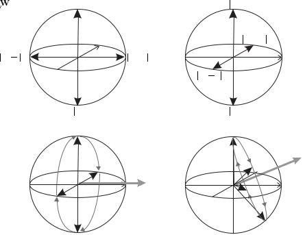
Fig. 7.2 The Bloch sphere. The position vectors of points on its surface represent the states of a two-level system (in Hilbert space). Examples of states are shown in (a) and (b). At the poles of the sphere the Bloch vector is R = w e3, with w = ±1 corresponding to the states |1 and |2 , respectively. States that lie on the equator of the Bloch sphere have the
form R = |
u e |
√ |
|
|
|
± |
correspond |
|
|
|
1 |
+ v e2, e.g. the states for which R = |
v e2 with u = 0 and v = 1 are shown in (b) and these |
|
|||
to (|1 ± i |2 )/ |
|
|
|
|||||
|
2, respectively (normalisation constants are not given in the figure for clarity). These examples illustrate an |
|||||||
interesting |
property of this representation of quantum states, namely that diametrically-opposite states on the Bloch sphere |
|||||||
|
|
|
|
|
|
|
||
are orthogonal. (c) The evolution of the Bloch vector for a system driven by a resonant field, i.e. δ = 0 so that W = Ω e1 in eqn 7.49. The evolution follows a great circle from 1 at the north pole to |2 at the south pole and back again, as described
|
in Example 7.1. The Bloch vector remains perpendicular to W. (d) When δ = 0 the Bloch vector also has a fixed angle with respect to W, since R · W = RW cos θ is constant, but θ is not equal to π/2. (This quantum mechanical description of the two-level atom is equivalent to that for a spin-1/2 system.)
132 The interaction of atoms with radiation
17In this particular example the fi- nal state is obvious by inspection, but clearly the same principles apply to
other |
initial |
states, |
e.g. states of the |
|||
|
|
iφ |
|
√ |
|
|
form |
|1 + e |
|
|2 / |
|
2 that lie on the |
|
equator of the sphere. The Bloch sphere is indispensable for thinking about more complex pulse sequences, such as those used in nuclear magnetic resonance (NMR).
energy −µ · B is constant, and the magnetic moment precesses around the direction of the field B = Bez . In the Bloch description the fictitious magnetic field lies along W and the magnitude W in eqn 7.28 determines the precession rate.
Example 7.1 Resonant excitation (δ = 0) gives W = Ω e1 and R describes a cone about e1. An important case is when all the population starts in level 1 so that initially R · e1 = 0; in this case the Bloch vector rotates in the plane perpendicular to e1 mapping out a great circle on the Bloch sphere, as drawn in Fig. 7.2(c). This motion corresponds to the Rabi oscillations (eqn 7.29). In this picture a π/2-pulse rotates the Bloch vector through π/2 about e1. A sequence of two π/2-pulses gives a π-pulse that rotates the Bloch vector (clockwise) through π aboute1, e.g. w = 1 → w = −1 and this represents the transfer of all the population from level 1 to 2.17 This is consistent with the more general statement given in eqn 7.30.
The very brief introduction to the Bloch sphere given in this section shows clearly that a two-level atom’s response to radiation does not increase indefinitely with the driving field—beyond a certain point an increase in the applied field (or the interaction time) does not produce a larger dipole moment or change in population. This ‘saturation’ has important consequences and makes the two-level system di erent from a classical oscillator (where the dipole moment is proportional to the field, as will be shown in Section 7.5).
18This assumes weak excitation:
|c2|2 1.
19This is not the FWHM but it is close enough for our purposes.
20This expression is equivalent to eqn 6.40 that was used to calculate the line width for an atomic clock.
7.4Ramsey fringes
The previous sections in this chapter have shown how to calculate the response of a two-level atom to radiation. In this section we shall apply this theory to radio-frequency spectroscopy, e.g. the method of magnetic resonance in an atomic beam described in Chapter 6. However, the same principles are important whenever line width is limited by the finite interaction time, both within atomic physics and more generally. In particular, we shall calculate what happens to an atom subjected to two pulses of radiation since such a double-pulse sequence has favourable properties for precision measurements.
An atom that interacts with a square pulse of radiation, i.e. an oscillating electric field of constant amplitude from time t = 0 to τp, and E0 = 0 otherwise, has a probability of excitation as in eqn 7.15.18 This excitation probability is plotted in Fig. 7.1 as a function of the radiation’s frequency detuning from the (angular) resonance frequency ω0. As stated below eqn 7.16, the frequency spread given by the first minimum of the sinc2 function corresponds to a width19
∆f = |
∆ω |
= |
1 |
. |
(7.50) |
2π |
|
||||
|
|
τp |
|
||
The frequency spread is inversely proportional to the interaction time,20

as expected from the Fourier transform relationship of the frequency and time domains.
We shall now consider what happens when an atom interacts with two separate pulses of radiation, from time t = 0 to τp and again from t = T to T + τp. Integration of eqn 7.10 with the initial condition c2 = 0 at t = 0 yields
|
Ω |
|
1 |
− |
exp[i(ω |
ω)τ ] |
|
|
|
|
||
c2 (t) = |
|
|
|
0 − |
p |
|
|
|
|
|||
2 |
|
|
|
ω0 − ω |
1 |
|
exp[i(ω |
ω)τ ] |
(7.51) |
|||
|
|
|
|
|
|
|
|
. |
||||
|
|
|
|
|
|
+ exp[i(ω0 − ω)T ] |
|
− |
0 − |
p |
||
|
|
|
|
|
|
|
|
|||||
|
|
|
|
|
|
|
|
ω0 − ω |
|
|||
This is the amplitude excited to the upper level after both pulses (t > T + τp). The first term in this expression is the amplitude arising from the first pulse and it equals the part of eqn 7.14 that remains after making the rotating-wave approximation.21 Within this approximation, interaction with the second pulse produces a similar term multiplied by a phase factor of exp[i(ω0 −ω)T ]. Either of the pulses acting alone would a ect the system in the same way, i.e. the same excitation probability |c2|2 as in eqn 7.15. When there are two pulses the amplitudes in the excited state interfere giving
|
|
Ω |
sin |
|
(ω0 |
ω)τp/2 |
|
|
2 |
|
|
|
||||
|
|
|
|
|
|
|
|
|||||||||
|c2|2 = |
|
|
{ |
− |
|
|
} |
× |1 + exp[i(ω0 − ω)T ]|2 |
|
|||||||
|
|
|
(ω0 |
ω) |
|
|
|
|||||||||
|
|
|
Ωτp |
|
2 |
|
− |
|
|
2 |
|
δ T |
|
|||
|
|
|
|
|
|
sin (δ τp/2) |
|
|
|
2 |
|
|||||
|
= |
|
|
|
|
|
3 |
|
|
4 |
cos |
|
, |
(7.52) |
||
|
2 |
|
δ τp/2 |
|
||||||||||||
|
|
|
|
|
|
2 |
|
|||||||||
where δ = ω |
|
|
0 |
|
|
|
|
frequency detuning. The double-pulse sequence |
||||||||
|
ω |
is the |
||||||||||||||
|
− |
|
|
|
|
|
|
|
|
|
|
|
|
|
|
|
produces a signal of the form shown in Fig. 7.3. These are called Ramsey fringes after Norman Ramsey and they have a very close similarity to the interference fringes seen in a Young’s double-slit experiment in optics— Fraunhofer di raction of light with wavevector k from two slits of width a and separation d leads to an intensity distribution as a function of angle θ given by22
I = I0 cos2 |
|
1 |
kd sin θ sinc2 |
|
1 |
ka sin θ . |
(7.53) |
2 |
2 |
The overall envelope proportional to sinc2 comes from single-slit di raction. The cos2 function determines the width of the central peak in both eqns 7.53 and 7.52.23
For the atom excited by two pulses of radiation the excitation drops from the maximum value at ω = ω0 to zero when δ T /2 = π/2 (or to half the maximum at π/4); so the central peak has a width (FWHM) of
∆ω = π/T , or equivalently |
|
|
|
∆f = |
1 |
. |
(7.54) |
|
|||
2T |
This shows that Ramsey fringes from two interactions separated by time T have half the width of the signal from a single long interaction of
7.4Ramsey fringes 133
21Neglecting terms with ω0 + ω in the denominator.
22See Section 11.1 and Brooker (2003).
23In both quantum mechanics and optics, the amplitudes of waves interfere constructively, or destructively, depending on their relative phase. Also, the calculation of Fraunhofer di raction as a Fourier transform of amplitude in the plane of the object closely parallels the Fourier transform relationship between pulses in the time domain and the frequency response of the system.
134 The interaction of atoms with radiation
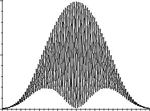
Fig. 7.3 Ramsey fringes from an atomic fountain of caesium, showing
the transition probability for the F = 3, MF = 0 to F = 4, MF = 0 transition versus the frequency of the mi-
crowave radiation in the interaction region. The height of the fountain is 31 cm, giving a fringe width just below 1 Hz (i.e. ∆f = 1/(2T ) = 0.98 Hz, see text)—the envelope of the fringes has a more complicated shape than that derived in the text, but this has little influence since, during operation as a frequency standard, the microwaves have a frequency very close to the centre which, by definition, corresponds to 9 192 631 770 Hz. This is real experimental data but the noise is not visible because the signal-to-noise ratio is about 1000 (near the centre), and with such an extremely high-quality signal the short-term stability of a microwave
source referenced to the caesium transition is about 1 × 10⁻¹³ for 1 s of av-
eraging. Courtesy of Dale Henderson, Krzysztof Szymaniec and Chalupczak Witold, National Physical Laboratory, Teddington, UK.
24Ramsey originally introduced two separated interactions in an atomicbeam experiment to avoid the line broadening by inhomogeneous magnetic fields. A small phase di erence between the two interaction regions just causes a phase shift of the fringes, whereas if the atom interacts with the radiation throughout a region where the field varies then the contributions from each part of the interaction region do not add in phase. The phasor description, commonly used in optics, gives a good way of thinking about this—Young’s fringes have a high contrast when the two slits of separation d are illuminated coherently, but to achieve the di raction limit from a single wide slit of width d requires a good wavefront across the whole aperture.
25In the Bloch sphere description this corresponds to the following path: the initial π/2-pulse causes e3 → e2, then the accumulated phase causes the state vector to move around the equator of the sphere to −e2, from whence the fi- nal π/2-pulse takes the system back up to e3 (see Fig. 7.2). This formalism allows quantitative calculation of the fi- nal state for any type of pulse.
|
1.0 |
|
|
|
|
|
|
|
|
probability |
0.5 |
|
|
|
|
|
|
|
|
Transition |
|
|
|
|
|
|
|
|
|
|
|
|
|
|
|
|
|
|
|
|
0.0−80 |
−60 |
−40 |
−20 |
0 |
20 |
40 |
60 |
80 |
|
|
Frequency of microwaves relative to line centre (Hz) |
|
||||||
duration T (cf. eqn 7.50); also, it is often preferable to have two separated interaction regions, e.g. for measurements in an atomic fountain as described in Chapter 8.24
In practice, microwave experiments use strong rather than weak excitation (as assumed above) to obtain the maximum signal, i.e. |c2|2 1. This does not change the width of the Ramsey fringes, as shown by considering two π/2-pulses separated by time T . If no phase shift accumulates between the two pulses they add together to act as a π-pulse that transfers all the population to the upper state—from the north to the south pole of the Bloch sphere, as shown in Fig. 7.2(c). But if a relative phase shift of π accrues during the time interval T then there is destructive interference between the amplitudes in the upper state produced by the two pulses.25 Thus the first minimum from the central fringe occurs for δ T = π, which is the condition that gave eqn 7.54, and so that equation remains accurate.
7.5Radiative damping
This section shows how damping a ects the coherent evolution of the Bloch vector described in the previous section. It is shown by analogy with the description of a classical dipole that a damping term should be introduced into eqns 7.46. Ultimately, such an argument by analogy is only a justification that the equations have an appropriate form rather

7.5 Radiative damping 135
than a derivation, but this approach does give useful physical insight.
7.5.1The damping of a classical dipole
Damping by spontaneous emission can be introduced into the quantum treatment of the two-level atom, in a physically reasonable way, by comparison with the damping of a classical system. To do this we first review the damped harmonic oscillator and express the classical equations in a suitable form. For a harmonic oscillator of natural frequency ω0, Newton’s second law leads to the equation of motion
.. . |
2 |
F (t) |
|
|
x + βx + ω0 x = |
|
cos ωt . |
(7.55) |
|
|
||||
|
|
m |
|
|
The driving force has amplitude F (t) that varies slowly compared to the
.
oscillation at the driving frequency. (The friction force is Ffriction = −αx
and β = α/m, where m is the mass.) To solve this we look for a solution of the form
x = U (t) cos ωt − V (t) sin ωt . |
(7.56) |
This anticipates that most of the time dependence of the solution is an oscillation at frequency ω, and U is the component of the displacement
phase with the force, and the quadrature component |
V |
has a phase |
||||
in- |
26 |
of π/2 with respect to F cos ωt. |
27 |
|
|
|
lead |
|
|
Substitution of eqn 7.56 into |
|||
eqn 7.55 and equating terms that depend on sin ωt and cos ωt gives |
||||||
. |
β |
|
|
|
|
|
U = (ω − ω0) V − |
|
U , |
|
|
||
2 |
|
(7.57) |
||||
. |
|
|
β |
F (t) |
||
|
|
|
||||
V = − (ω − ω0) U − |
|
V − |
|
, |
||
2 |
2mω |
|||||
respectively. The amplitudes U and V change in time as the amplitude of the force changes, but we assume that these changes occur slowly
compared to the fast oscillation at ω. This slowly-varying envelope ap-
.. ..
proximation has been used in the derivation of eqn 7.57, i.e. U and V have
.
been neglected and V ωV (see Allen and Eberly 1975). By setting
. .
U = V = 0 we find the form of the solution that is a good approximation when the amplitudes and the force change slowly compared to the damping time of the system 1/β:
U |
= |
|
ω0 − ω |
|
|
F |
|
, |
|
(7.58) |
|||
|
(ω − ω0)2 + (β/2)2 2mω |
|
|||||||||||
|
|
|
|
|
|
||||||||
V |
= |
|
−β/2 |
|
|
|
F |
. |
|
|
(7.59) |
||
|
|
|
|
|
|
|
|||||||
|
(ω − ω0)2 + (β/2)2 2mω |
|
|
|
|
||||||||
The approximation ω2 |
2 |
|
|
|
|
|
|
|
|
ω |
) has |
||
|
|
− ω0 = (ω + ω0) (ω − ω0) |
|
2ω (ω −28 0 |
|
||||||||
been used so these expressions are only valid close to resonance |
—they |
||||||||||||
give the wrong result for ω 0. The phase is found from tan φ = V/U (see Exercise 7.7). The phase lies in the range φ = 0 to −π for a force of constant amplitude.29
26A phase lead occurs when V(t) > 0, since −sin ωt = cos(ωt + π/2), and V(t) < 0 corresponds to a phase lag.
27This method of considering the components U and V is equivalent to the phasor description which is widely used in the theory of a.c. circuits (made from capacitors, inductors and resistors) to represent the phase lag, or lead, between the current and an applied voltage of the form V0 cos ωt.
28This is a very good approximation
for optical transitions since typically β/ω0 10−6. The assumption of small damping is implicit in these equations and therefore the resonance frequency is very close to ω0.
29It is well known from the study of the harmonic oscillator with damping that the mechanical response lags behind the driving. At low frequencies the system closely follows the driving force, but above the resonance, where
ω > ω0, the phase shift lies in the range
−π/2 < ϕ < −π.