Atomic physics (2005)

30For light damping (β/ω0 1) the

decaying oscillations have angular frequency ω = ω02 − β2/4 1/2 ω0.

31We use the same slowly varying envelope approximation. as for eqn 7.57, namely V ωV, etc.

32This is normally a positive quantity since r < 0 (see eqn 7.59).

33See Fig. 9.12.

For no driving force (F = 0) the energy decays away. This is consistent with the complementary function of eqn 7.55 (the solution for F = 0) that gives the oscillator’s transient response as30

Energy is proportional to the amplitude of the motion squared, hence the exp (−βt/2) dependence in eqn 7.61 becomes E exp (−βt). The term F Vω/2 in eqn 7.60 is the rate at which the driving force does work on the oscillator; this can be seen from the following expression for power as the force times the velocity:

The overlining indicates an average over many periods of the oscillation at ω, but the amplitude of the force F (t) may vary (slowly) on a longer time-scale. Di erentiation of eqn 7.56 gives the velocity as31

This shows that absorption of energy arises from the quadrature component of the response V.

In the classical model of an atom as an electron that undergoes simple harmonic motion the oscillating electric field of the incident radiation produces a force F (t) = −e|E0| cos ωt on the electron. Each atom in the sample has an electric dipole moment of D = −ex (along the direction of the applied field). The quadrature component of the dipole that gives absorption has a Lorentzian function of frequency as in eqn 7.59. The in-phase component of the dipole that determines the polarization of the medium and its refractive index (Fox 2001) has the frequency dependence given in eqn 7.58.33

When any changes in the driving force occur slowly eqn 7.60 has the

This shows that the energy of the classical oscillator increases linearly with the strength of the driving force, whereas in a two-level system the energy has an upper limit when all the atoms have been excited to the upper level.

A two-level atom has an energy proportional to the excited-state population, E = ρ22 ω0. By analogy with eqn 7.60 for the energy of a classical oscillator, we introduce a damping term into eqn 7.44 to give

In the absence of the driving term (Ω = 0) this gives exponential decay of the population in level 2, i.e. ρ22(t) = ρ22(0) exp (−Γt). In this analogy, between the quantum system and a classical oscillator, Γ corresponds to β. From eqns 7.57 we see that the coherences u and v have a damping factor of Γ/2 and eqns 7.46 become the optical Bloch equations34

For Ω = 0 the population di erence w → 1. These optical Bloch equations describe the excitation of a two-level atom by radiation close to resonance for a transition that decays by spontaneous emission. There is not room here to explore all of the features of these equations and their many diverse and interesting applications; we shall concentrate on the steady-state solution that is established at times which are long compared to the lifetime of the upper level (t Γ−1), namely35

These show that a strong driving field (Ω → ∞) tends to equalise the populations, i.e. w → 0. Equivalently, the upper level has a steady-state population of

→ 1/2 as the intensity increases. This key result is used in Chapter 9 on radiation forces.

In the above, the optical Bloch equations have been justified by analogy with a damped classical oscillator but they also closely resemble the Bloch equations that describe the behaviour of a spin-1/2 particle in a combination of static and oscillating magnetic fields.36 The reader familiar with magnetic resonance techniques may find it useful to make an analogy with that historically important case.37 For times much shorter than any damping or relaxation time, the two-level atom and spin-1/2 system behave in the same way, i.e. they have a coherent evolution such as π- and π/2-pulses, etc. A steady-state solution of the optical Bloch equations has been presented (and nothing has been said about the different result for a spin-1/2 system).

34The main purpose of the rather lengthy discussion of the classical case was to highlight the correspondence between u, v and U, V to make this step seem reasonable. An auxiliary feature of this approach is to remind the reader of the classical electron oscillator model of absorption and dispersion (which is important in atomic physics).

35The steady. -state. solution. is obtained by setting u = v = w = 0 in eqns 7.67 to give three simultaneous equations.

36The Zeeman e ect leads to a splitting between states with ms = ±1/2 to give a two-level system, and the oscillating magnetic field drives magnetic dipole transitions between the levels. In atomic physics such transitions occur between Zeeman states and hyperfine levels (Chapter 6).

37The Bloch equations were well known from magnetic resonance techniques before lasers allowed the observation of coherent phenomena in optical transitions. Radio-frequency transitions have negligible spontaneous emission and the magnetic dipole of the whole sample decays by other mechanisms. Where the optical Bloch equations (eqns 7.67) have decay constants of Γ and Γ/2 for the population and coherences, respectively, the Bloch equations have 1/T1 and 1/T2. The decay rates 1/T1 and 1/T2 in magnetic resonance techniques are expressed in terms of T1 and T2, the longitudinal and transverse relaxation times, respectively. Under some conditions the two relaxation times are similar, but in other cases T2 T1. T1 describes the relaxation of the component of the magnetic moment parallel to the applied field B which requires exchange of energy (e.g. with the phonons in a solid). T2 arises from the dephasing of individual magnetic moments (spins) so that the magnetisation of the sample perpendicular to B decays. For further details see condensed matter texts, e.g. Kittel (2004).

38N represents the number density and has dimensions of m−3, following the usual convention in laser physics.

Monochromatic radiation causes an atom to undergo Rabi oscillations, but when the transition has damping the atom settles down to a steady state in which the excitation rate equals the decay rate. This has been shown explicitly above for an optical transition with spontaneous emission, but the same reduction of the coherent evolution of quantum amplitudes to a simple rate equation for populations (amplitudes squared) also occurs for other line-broadening mechanisms, e.g. Doppler broadening (Chapter 8) and collisions. Thus the equilibrium situation for monochromatic radiation is described by rate equations like those in Einstein’s treatment of excitation by broadband radiation (eqns 1.25). It is convenient to write these rate equations in terms of an optical absorption cross-section defined in the usual way, as in Fig. 7.4. Consider a beam of particles (in this case photons) passing through a medium with

Natoms per unit volume.38 A slab of thickness ∆z has N ∆z atoms per unit area and the fraction of particles absorbed by the target atoms is

Nσ∆z, where σ is defined as the cross-section; N σ∆z gives the fraction of the target area covered by the atoms and this equals the probability that an incident particle hits an atom in the target (as it passes through the slab). The parameter σ that characterises the probability of absorption is equally well definable in quantum mechanics (in which photons and particles are delocalised, fuzzy objects) even though this cross-section generally has little relation to the physical size of the object (as we shall see). The probability of absorption equals the fraction of intensity lost, ∆I/I = −N σ∆z, so the attenuation of the beam is described by

This formula, known as Beer’s law (see Fox 2001), works well for absorption of low-intensity light that leaves most of the population in the ground state. Intense laser light significantly a ects the populations of the atomic levels and we must take this into account. Atoms in level 2 undergo stimulated emission and this process leads to a gain in intensity (amplification) that o sets some of the absorption. Equation 7.70 must be modified to39

dI

dz

(7.72)

Absorption and stimulated emission have the same cross-section. For the specific case of a two-level atom this can be seen from the symmetry with respect to the exchange of the labels 1 and 2 in the treatment of the two-level atom in the early parts of this chapter; the oscillating electric field drives the transition from 1 to 2 at the same rate as the reverse process—only the spontaneous emission goes one way. This is an example of the general principle that a strong absorber is also a strong emitter.40 This is also linked to the equality of the Einstein coe cients, B12 = B21, for non-degenerate levels. The population densities in the two levels obey the conservation equation N = N1 + N2.41 In the steady state conservation of energy per unit volume of the absorber requires that

On the left-hand side is the amount by which the rate of absorption of energy exceeds the stimulated emission, i.e. the net rate of energy absorbed per unit volume. On the right-hand side is the rate at which the atoms scatter energy out of the beam—the rate of spontaneous emission for atoms in the excited state times ω.42 The number densities are related to the variables in the optical Bloch equations by ρ22 = N2/N and

π2c2

σ (ω) = 3 × (7.76)

ω02

The Lorentzian frequency dependence is expressed by the line shape function

1Γ

gH (ω) = 2π (ω − ω0)2 + Γ2/4 , (7.77) where the subscript H denotes homogeneous, i.e. something that is the same for each atom, like the radiative broadening considered here.44 The

39We do not try to include the degeneracy of the levels because illumination with intense polarized laser light usually leads to unequal populations of the

states with di erent MJ , or MF . This di ers from the usual situation in laser physics where the excitation, or pumping mechanisms, populate all states in a given level at the same rate, so N1/g1 and N2/g2 can be taken as the population densities per state. Selective excitation of the upper level can give N2/g2 > N1/g1, and hence gain.

40The laws of thermodynamics require that an object stays in equilibrium with black-body radiation at the same temperature, hence the absorbed and emitted powers must balance.

41Compare this with eqns 1.26, 7.7 and

42This assumes that atoms do not get rid of their energy in any other way such as inelastic collisions.

43Intensity is related to the electric

field amplitude by I = 0c |E0 (ω)|2 /2, and Ω2 = e2X122 |E0|2 / 2 (eqn 7.12).

Also X122 = |D12|2 /3 A21 (eqn 7.23). The degeneracy factors are g1 = g2 = 1

for the two-level atom, but see eqn 7.79.

44It is a general result that homogeneous broadening mechanisms give a Lorentzian line shape.

45Spontaneously emitted photons go in random directions so an average over angles always occurs in the calculation of A21.

The pre-factor of 3 in eqn 7.76 may have any value in the range 0 to 3. It has the maximum value of 3 for atoms with the optimum orientation to absorb a beam of polarized laser light (from a specific direction). However, if either the light is unpolarized or the atoms have a random orientation (i.e. they are uniformly distributed across all the MJ states or MF states) then the pre-factor is 1 because |X12|2 = |D12|2 /3 as in eqn 7.21 (from the average of cos2 θ over all angles), and this 1/3 cancels the pre-factor of 3.45 Under these conditions the absorption does not depend on the magnetic state (MJ or MF ) so a real atom with degenerate levels has a cross-section of

46Typically, for atoms with a welldefined orientation the polarization of the light is chosen to give the maximum cross-section. If this is not the case then the angular momentum algebra may be required to calculate the matrix elements. Only in special cases would the polarization be chosen to give a very weak interaction, i.e. a pre-factor much less than unity in eqn 7.76.

This equation, or eqn 7.76, applies to many experimental situations. Careful study of the following examples gives physical insight that can be applied to other situations.46

Example 7.2 Atoms in a specific MF state interacting with a polarized laser beam, e.g. sodium atoms in a magnetic trap that absorb a circularlypolarized probe beam (Fig. 7.5)

This gives e ectively a two-level system and the polarization of the light matches the atom’s orientation so eqn 7.76 applies (the pre-factor has the maximum value of 3). To drive the ∆MF = +1 transition the

circularly-polarized light must have the correct handedness and propagate along the atom’s quantisation axis (defined by the magnetic field in this example).47

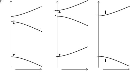
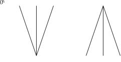
Example 7.3 The absorption of light on an s–p transition, e.g. the 3s–3p resonance line of sodium

Light with a particular polarization and direction drives a transition to one magnetic sub-level in the upper level, as shown in Fig. 7.6(a). Since the lower level has only ml = 0 there is no averaging over the orientation and eqn 7.76 applies. Unpolarized light drives transitions to the three upper ml states equally. For each transition the averaging gives a factor of 1/3 but all three transitions contribute equally to the absorption so the atoms have the same cross-section as for polarized light (eqn 7.79 with g2/g1 = 3). Thus the s–p transition is a special case that gives the same absorption cross-section whatever the polarization of the light. Atoms with ml = 0 have no preferred direction and interact in the same way with light of any polarization (or direction). In contrast, for the p–s transition shown in Fig. 7.6(b), atoms in a given ml state only interact with light that has the correct polarization to drive the transition to ml = 0.

47The direction of the electric field at the atom depends on both the polarization and direction of the radiation, e.g. circularly-polarized light that propagates perpendicular to the quantisation axis drives ∆MF = 0 and ±1 (π- and σ-) transitions. This leads to a smaller cross-section than when the light propagates along the axis. Radiation that propagates in all directions does not produce a polarized electric field, e.g. isotropic radiation in a blackbody enclosure.

Fig. 7.6 A comparison of s–p and p–s transitions. (a) The three transitions a, b and c between the s and p levels have equal strength. The physical reason for this is that the spontaneous decay rate of the upper ml states cannot depend on the atom’s orientation in space. Light linearly-polarized parallel to the z-axis drives π-transition b only, and spontaneous decay occurs back to the initial state since there are no other accessible states—this gives the equivalent of a two-level system. The s–p transition is a special case where the absorption does not depend on the polarization, e.g. unpolarized light gives equal excitation rates on the three transitions a, b and c, and this increases the absorption by the degeneracy factor g2/g1 = 3, thereby cancelling the 1/3 that arises in the orientational average. (b) In contrast, for the p–s transition the peak cross-section is one-ninth of that in (a).48

48Spin is ignored here. This applies when either the fine structure is not resolved, e.g. this may arise for the transition 2s–3p in hydrogen where the fine structure of the upper level is small, or to transitions between singlet terms, i.e. 1S–1P and 1P–1S (with ml → Ml in the figure).

49This equation is very similar to the formula for the saturation of gain in a homogeneously-broadened laser system since gain is negative absorption.

50Here Isat = ωA21/ (2σ(ω0)) and σ(ω0) is given by eqn 7.81.

In a two-level atom the upper level can only decay to level 1 so Γ = A21, and for a transition of wavelength λ0 = 2πc/ω0 we find

This maximum cross-section is much larger than the size of the atom, e.g. the λ0 = 589 nm transition of sodium has σ (ω0) = 2 × 10−13 m2, whereas in kinetic theory the atoms have a cross-section of only πd2 = 3×10−18 m−2 for an atomic diameter of d = 0.3 nm—‘collisions’ between atoms and photons have a large resonant enhancement. The optical cross-section decreases rapidly o resonance, e.g. light of wavelength 600 nm gives Γ/ (ω − ω0) = 10−6 for the sodium transition above, so that σ (ω) = 10−12 × σ (ω0) = 2 × 10−25 m2. Clearly the absorption of radiation has little relation to the size of the electronic orbitals.

7.6.2The saturation intensity

In the previous section we calculated the absorption cross-section starting from eqn 7.73 and we shall now use the same equation to determine the population di erence; we can write eqn 7.73 as (N1 − N2) × r = N2, where the dimensionless ratio r = σ (ω) I (ω) /( ωA21). This equation and N1 + N2 = N give the di erence in population densities as

where the saturation intensity is defined by

It is important to note that other definitions of saturation intensity are also used, such as the above expression without 2 in the denominator. From eqn 7.72 we find that the absorption coe cient depends on intensity as follows:49

The minimum value of Isat (ω) occurs on resonance where the crosssection is largest; this minimum value is often referred to as the saturation intensity, Isat ≡ Is (ω0), given by50

where τ = Γ−1 is the lifetime for radiative broadening. For example, the resonance transition in sodium at λ = 589 nm has a lifetime of τ = 16 ns and for an appropriate polarization (as in Fig. 7.5) the atom cycles on an e ectively two-level transition. This leads to an intensity Isat = 60 W m−2, or 6 mW cm−2, that can easily be produced by a tunable dye laser.

We can also obtain eqn 7.82 directly from the steady-state value of w = (N1 − N2)/N in eqn 7.68 if the saturation intensity is defined by

This is equivalent to eqn 7.85.51 At saturation the Rabi frequency has a value comparable with Γ.

51As discussed after eqn 7.75, Ω2/I does not depend on the electric field.

7.6.3Power broadening

Equation 7.84 for κ (ω, I) contains two quantities that vary with frequency: σ(ω) and Is(ω).52 Rearranging this equation to show the frequency dependence, and defining σ0 ≡ σ(ω0) as the maximum crosssection in eqn 7.81, we find that

52In terms of the minimum value Isat = Is (ω0) we can rewrite eqn 7.83

as

Is (ω) = σ0 .

Γ2/4 σ (ω) = σ0 (ω − ω0)2 + Γ2/4 .

The expression for the absorption coe cient κ (ω, I) has a Lorentzian line shape with a full width at half maximum (FWHM) of

The line width increases with intensity. This power broadening occurs because saturation reduces the absorption near the resonance while far from resonance the absorption changes little (see Fig. 7.7). The expression for the population in the upper level ρ22 in eqn 7.69 also has the same power-broadened line width, as in eqn 7.88.53 The relationship between this absorption and the populations of the two levels is discussed in Exercise 7.11.

53This can be shown by rearrangement of the denominator of eqn 7.69 in terms of a line width

Fig. 7.7 The absorption coe cient κ(ω, I) is a Lorentzian function of the frequency that peaks at ω0, the atomic resonance. Saturation causes the absorption line shape to change from the curve for a low intensity (I Isat, dashed line), to a broader curve (solid line), with a lower peak value, described by the Lorentzian function in eqn 7.87.

Fig. 7.8 The treatment of the interaction of a two-level atom with radiation by time-dependent perturbation theory leads to eqn 7.89, that looks similar to a time-independent perturbation (proportional to Ω) of two energy levels with an energy separation of δ. The light shift is the di erence between the unperturbed energies and energy eigenvalues of the system when it is perturbed by the radiation.

This result of time-dependent perturbation theory closely resembles the equations for a time-independent perturbation of two states with an energy separation of δ (see Appendix A); the two states are the excited state at E2 and a level at energy E1 + ω, corresponding to the ground state plus a photon of the radiation field, see Fig. 7.9. This system of atom plus photon is called a ‘dressed atom’—see Cohen-Tannoudji et al. (1992) for a much more in-depth treatment.

Normally light shifts are most important at large frequency detuning where the e ect of absorption is negligible; in this case |δ| Ω and the

The states are shifted from their unperturbed eigenfrequencies by the light shift ±Ω2/4δ. From eqn 7.89 we see that the amplitude c1 is associated with the state with unperturbed energy +δ/2 and lies above

Light

shift

Unperturbed

Perturbed

7.8Comment on semiclassical theory

This chapter’s treatment of the interaction of radiation with atoms is semiclassical—the energy of the atoms is quantised but the radiation is not (since E0 cos ωt is a classical electric field). It is individual two-level atoms that absorb energy in lumps of ω from the radiation; nevertheless, the quantity I/ ω is commonly referred to as the flux of photons. In addition to transitions between two bound quantum states of the atom, this semiclassical theory can also describe photo-ionization where light excites an electron from a bound state to an unbound state above the ionization limit. In such a transition the atom suddenly becomes an ion (plus a free electron) at a given time, like a quantum jump between bound states. The average of many such jumps corresponds to the rate predicted semiclassically.54 Photo-ionization of individual atoms closely resembles the photoelectric e ect that occurs at the surface of a metal with work function Φ illuminated by light of frequency ω. The sur-

54Similarly, in radioactivity the individual nuclei decay randomly but a large sample exhibits a smooth exponential decay.