Atomic physics (2005)

Exercises

in units of cm−1. Devise an extrapolation procedure to find the ionization limit of sodium with a precision justified by the data. Convert the result into electron volts. (You may find a spreadsheet program useful for manipulating the numbers.)

What is the e ective principal quantum number n of the valence electron in the ground configuration?

(4.3) Quantum defects of sodium

The binding energies of the 3s, 4s, 5s and 6s configurations in sodium are 5.14 eV, 1.92 eV, 1.01 eV and 0.63 eV, respectively. Calculate the quantum defects for these configurations and comment on what you find.

Estimate the binding energy of the 8s configuration and make a comparison with the n = 8 shell in hydrogen.

(4.4) Quantum defect

Estimate the wavelength of laser radiation that excites the 5s 2S1/2–7s 2S1/2 transition in rubidium by simultaneous absorption of two photons with the same frequency (IE(Rb) = 4.17 eV). (Twophoton spectroscopy is described in Section 8.4 but specific details are not required here.)

(4.5) Application of quantum defects to helium and helium-like ions

(a)Calculate the wavelength of the 1s2p–1s3d line in helium and compare it with the Balmer-α line in hydrogen.

(b)Calculate the quantum defects for the configurations of helium in the table. Estimate the binding energies of the 1s4l configurations.

(c)The levels belonging to the 1s4f configuration of the Li+ ion all lie at an energy of 72.24 eV above the ion’s ground state. Estimate the second ionization energy of this ion. Answer: 75.64 eV.

(4.6) Quantum defects and fine structure of potassium

An atomic vapour of potassium absorbs light at the wavelengths (in nm): 769.9, 766.5, 404.7, 404.4, 344.7 and 344.6. These correspond to the transitions from the ground configuration 4s. Explain these observations as fully as you can and estimate the mean wavelength of the next doublet

in the series, and its splitting. (Potassium has IE = 4.34 eV.)28

(4.7) The Z-scaling of fine structure

Calculate the fine-structure splitting of the 3p configuration of the hydrogen-like ion Na+10 (in eV).

Explain why it is larger than the fine structure of the same configuration in the neutral sodium (0.002 eV) and hydrogen (1.3 × 10−5 eV).

(4.8) Relative intensities of fine-structure components

(a)An emission line in the spectrum of an alkali has three fine-structure components cor-

responding to the transitions 2P3/2–2D3/2, 2P3/2–2D5/2 and 2P1/2–2D3/2. These components have intensities a, b and c, respectively,

that are in the ratio 1 : 9 : 5. Show that these satisfy the rule that the sum of the intensities of the transitions to, or from, a given level is proportional to its statistical weight (2J + 1).

(b)Sketch an energy-level diagram of the finestructure levels of the two terms nd 2D and n f 2F (for n > n). Mark the three allowed electric dipole transitions and find their relative intensities.

numerical calculations are carried out in a simple case that can be implemented easily on a computer with readily available spreadsheet programs.29 Of course, the properties of hydrogen-like atoms are well known and so the first stage really serves as a way of testing the numerical method (and checking that the formulae have been typed correctly). It is straightforward to extend the numerical method to deal with other cases, e.g. the potentials in the central-field approximation illustrated in Fig. 4.7.30

(a)Derivation of the equations

Show from eqn 2.4, and other equations in Chapter 2, that

turned into dimensionless variables: x = r/a0 and E is the energy in units of e2/8π 0a0 = 13.6 eV (equal to half the atomic unit of en-

quantum number.

The derivatives of a function f (x) can be approximated by

where δ is a small step size.32

Show that the second derivative follows by applying the procedure used to obtain the first derivative twice. Show also that substitution into eqn 4.14 gives the following expression for the value of the function at x + δ in terms of its value at the two previous points:

$ &

% − % 2

R(x + δ) = 2R(x) + V (x) E R(x)δ

'

− 1 − xδ R(x − δ) 1 + xδ .

(4.16) If we start the calculation near the origin then

etc. Note that in the first equation the value of R (x) at x = 2δ depends only on R (δ)—it can easily be seen why by inspection of eqn 4.16 for the case of x = δ (for this value of x the coe cient of R (0) is zero). Thus the calculation starts at x = δ and works outwards from there.33 At all other positions (x > δ) the value of the function depends on its values at the two preceding points. From these recursion relations we can calculate the function at all subsequent points.

The calculated functions will not be normalised and the starting conditions can be multiplied by an arbitrary constant without a ecting the eigenenergies, as will become clear from looking at the results. In the following R (δ) = 1 is the suggested choice but any starting value works.

(b)Implementation of the numerical method using a spreadsheet program

Follow these instructions.

1.Type the given text labels into cells A1, B1, C1, D2, E2 and F2 and the three numbers into cells D1, E1 and F1 so that it has the following form:

78 The alkalis

Column A will contain the x-coordinates, the potential will be in column B and the function in column C. Cells D1, E1 and F1 contain the step size, energy and orbital angular momentum quantum number (l = 1), respectively.

2.Put 0 into A2 and the formula =A2+$D$1 into A3. Copy cell A3 to the block A4:A1002. (Or start with a smaller number of steps and adjust D1 accordingly.)

3.The potential diverges at x = 0 so type inf. into B2 (or leave it blank, remembering not to refer to it).

Put the formula

=-2/A3 +$F$1*($F$1+1)/(A3*A3)

into cell B3 (as in eqn 4.15). Copy B3 into the block B4:B1002.

4.This is the crucial stage that calculates the function. Type the number 1 into cell C3. (We leave C2 blank since, as explained above, the value of the function at x = 0 does not a ect the solution given by the recursion relation in eqn 4.16.) Now move to cell C4 and enter the following formula for the recursion relation:

=( 2*C3+(B3-$E$1)*C3*$D$1*$D$1

- (1-$D$1/A3)*C2 )/ (1+$D$1/A3).

Copy this into the block C5:C1002. Create an xy-plot of the wavefunction (with data points connected by smooth lines and no markers); the x series is A2:A1002 and the y series is C2:C1002. Insert this graph on the sheet.

5.Now play around with the parameters and observe the e ect on the wavefunction for a particular energy.

(i)Show that the initial value of the function does not a ect its shape, or the eigenenergy, by putting 0.1 (or any number) into cell C3.

(ii)Change the energy, e.g. put -0.251 into cell E1, then -0.249, and observe the change in behaviour at large

x. (The divergence is exponential, so even a small energy discrepancy gives a large e ect.) Try the di erent energies again with bigger and smaller step sizes in D1. It is important to search for the eigenenergy using an appropriate range of x. The eigenenergy lies between the two values of the trial energy that give opposite divergence, i.e. upwards and downwards on the graph.

(iii)Change F1 to 0 and find a solution for l = 0.

6.Produce a set of graphs labelled clearly with the trial energy that illustrate the principles of the numerical solution, for the two functions with n = 2 and two other cases. Compare the eigenenergies with the Bohr formula.

Calculate the e ective principal quantum number for each of the solutions, e.g. by putting =SQRT(-1/E1) in G1 (and the label n* in G2).

(The search for eigenenergies can be automated by exploiting the spreadsheet’s ability to optimise parameters subject to constraints (e.g. the ‘Goal Seek’ command, or similar). Ask the program to make the last value of the function (in cell C1002) have the value of zero by adjusting the energy (cell E1). This procedure can be recorded as a macro that searches for the eigenenergies with a single button click.)

7.Implement one, or more, of the following suggestions for improving the basic method described above.

(i)Find the eigenenergies for a potential that tends to the Coulomb potential (−2/x in dimensionless units) at long range, like those shown in Fig. 4.7, and show that the quantum defects for that potential depend on l but only weakly on n.

(ii)For the potential shown in Fig. 4.7(c) compare the wavefunction in the inner and outer regions for several di erent energies. Give a qualitative explanation of the observed behaviour.

(iii)Calculate the function P (r) = rR(r) by putting A3*C3 in cell D3 and copying this to the rest of the column.

Make a plot of P (r), R(r) and V (r) for at least two di erent values of n and l. Adjust the value in C3, as in stage 5(i), to scale the functions to convenient values for plotting on the same axes as the potential.

(iv)Attempt a semi-quantitative calculation of the quantum defects in the lithium atom, e.g. model VCF(r) as in Fig. 4.7(a) for some reasonable choice

of rcore.34

(v) Numerically calculate the sum of r2R2 (r) δ for all the values of the function and divide through by its square root to normalise the wavefunction. With normalised functions (stored in a column of the spread-

Web site:

http://www.physics.ox.ac.uk/users/foot

sheet) you can calculate the electric

dipole matrix elements (and their ratios), e.g. | 3p| r |2s |2 / | 3p| r |1s |2 =

36, as in Exercise 7.6 (not forgetting the ω3 factor from eqn 7.23).

(vi)Assess the accuracy of this numerical method by calculating some eigenenergies using di erent step sizes. (More sophisticated methods of numerical integration provided in mathematical software packages can be compared to the simple method, if desired, but the emphasis here is on the atomic physics rather than the computation. Note that methods that calculate higher derivatives of the function cannot cope with discontinuities in the potential.)

In this chapter we shall look at atoms with two valence electrons, e.g. alkaline earth metals such as Mg and Ca. The structures of these elements have many similarities with helium, and we shall also use the centralfield approximation that was introduced for the alkalis in the previous chapter. We start with the Hamiltonian for N electrons in eqn 4.2 and insert the expression for the central potential VCF (r) (eqn 4.3) to give

1Choosing S(r) to account for all the repulsion between the sphericallysymmetric core and the electrons outside the closed shells, and also within the core, leaves the repulsion between the two valence electrons, i.e. Hre e2/4π 0r12. This approximation highlights the similarity with helium (although the expectation value is evaluated with di erent wavefunctions). Although it simplifies the equations nicely, this is not the best approximation for accurate calculations—S(r) can be chosen to include most of the direct integral (cf. Section 3.3.2). For alkali metal atoms, which we studied in the last chapter, the repulsion between electrons gives a spherically-symmetric potential, so that Hre = 0.

2For two p-electrons we cannot ignore ml as we did in the treatment of 1snl configurations in helium. Configurations with one, or more, s-electrons can be treated in the way already described for helium but with the radial wavefunctions calculated numerically.

is the residual electrostatic interaction. This represents that part of the repulsion not taken into account by the central field. One might think that the field left over is somehow non-central. This is not necessarily true. For configurations such as 1s2s in He, or 3s4s in Mg, both electrons have spherically-symmetric distributions but a central field cannot completely account for the repulsion between them—a potential VCF(r) does not include the e ect of the correlation of the electrons’ positions that leads to the exchange integral.1 The residual electrostatic interaction perturbs the electronic configurations n1l1n2l2 that are the eigenstates of the central field. These angular momentum eigenstates for the two electrons are products of their orbital and spin functions |l1ml1 s1ms1 |l2ml2 s2ms2 and their energy does not depend on the atom’s orientation so that all the di erent ml states are degenerate, e.g. the configuration 3p4p has (2l1 + 1) (2l2 + 1) = 9 degenerate combinations of Yl1,m1 Yl2 ,m2 .2 Each of these spatial states has four spin functions associated with it, but we do not need to consider thirty-six degenerate states since the problem separates into spatial and spin parts, as in helium. Nevertheless, the direct approach would require diagonalising matrices of larger dimensions than the simple 2 × 2 matrix whose determinant was given in eqn 3.17. Therefore, instead of that brute-force approach, we use the ‘look-before-you-leap’ method that starts by finding the eigenstates of the perturbation Hre. In that representation, Hre is a diagonal matrix with the eigenvalues as its diagonal elements.

The interaction between the electrons, from their electrostatic repulsion, causes their orbital angular momenta to change, i.e. in the vector model l1 and l2 change direction, but their magnitudes remain constant. This internal interaction does not change the total orbital angular momentum L = l1 +l2, so l1 and l2 move (or precess) around this vector, as illustrated in Fig. 5.1. When no external torque acts on the atom, L has a fixed orientation in space so its z-component ML is also a constant of the motion (ml1 and ml2 are not good quantum numbers). This classical picture of conservation of total angular momentum corresponds to the quantum mechanical result that the operators L2 and Lz both commute

Actually, Hre also commutes with the individual spins s1 and s2 but we chose eigenfunctions of S to antisymmetrise the wavefunctions, as

in helium—the spin eigenstates for two electrons are ψspinA and ψspinS for S = 0 and 1, respectively.4 The quantum numbers L, ML, S and MS

have well-defined values in this Russell–Saunders or LS-coupling scheme. Thus the eigenstates of Hre are |LMLSMS . In the LS-coupling scheme the energy levels labelled by L and S are called terms (and there is degeneracy with respect to ML and MS ). We saw examples of 1L and 3L terms for the 1snl configurations in helium where the LS-coupling scheme is a very good approximation. A more complex example is an npn p configuration, e.g. 3p4p in silicon, that has six terms as follows:

terms: L = 1S, 1P, 1D, 3S, 3P, 3D .

The direct and exchange integrals that determine the energies of these terms are complicated to evaluate (see Woodgate (1980) for details) and here we shall simply make some empirical observations based on the terms diagrams in Figs 5.2 and 5.3. The (2l1 + 1) (2l2 + 1) = 9 degenerate states of orbital angular momentum become the 1 + 3 + 5 = 9 states of ML associated with the S, P and D terms, respectively. As in helium, linear combinations of the four degenerate spin states lead to triplet and one singlet terms but, unlike helium, triplets do not necessarily lie below singlets. Also, the 3p2 configuration has fewer terms than the 3p4p configuration for equivalent electrons, because of the Pauli exclusion principle (see Exercise 5.6).

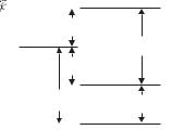
In the special case of ground configurations of equivalent electrons the spin and orbital angular momentum of the lowest-energy term follow some empirical rules, called Hund’s rules: the lowest-energy term has the largest value of S consistent with the Pauli exclusion principle.5 If

The LS-coupling scheme 81

Fig. 5.1 The residual electrostatic interaction causes l1 and l2 to precess around their resultant L = l1 + l2.

3The proof is straightforward for the quantum operator: Lz = l1z + l2z since

ml1 = q always occurs with ml2 = −q in eqn 3.30.

4The Hamiltonian H commutes with the exchange (or swap) operator Xij that interchanges the labels of the particles i ↔ j; thus states that are simultaneously eigenfunctions of both operators exist. This is obviously true for the Hamiltonian of the helium atom in eqn 3.1 (which looks the same if 1 ↔ 2), but it also holds for eqn 5.1. In general, swapping particles with the same mass and charge does not change the Hamiltonian for the electrostatic interactions of a system.

5Two electrons cannot both have the same set of quantum numbers.

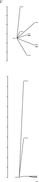
82 The LS-coupling scheme

Fig. 5.2 The terms of the 3p4p configuration in silicon all lie about 6 eV above the ground state. The residual electrostatic interaction leads to energy differences of 0.2 eV between the terms, and the fine-structure splitting is an order of magnitude smaller, as indicated for the 3P and 3D terms. This structure is well described by the LS-coupling scheme.

Fig. 5.3 The energies of terms of the 3p2 configuration of silicon. For equivalent electrons the Pauli exclusion principle restricts the number of terms— there are only three compared to the six in Fig. 5.2. The lowest-energy term is 3P, in accordance with Hund’s rules, and this is the ground state of silicon atoms.

6Hund’s rules are so commonly misapplied that it is worth spelling out that they only apply to the lowest term of the ground configuration for cases where there is only one incomplete subshell.

7The large total spin has important consequences for magnetism (Blundell 2001).

6.4

6.3

6.2

6.1

6.0

5.9

5.8

2.0

1.8

1.6

1.4

1.2

1.0

0.8

0.6

0.4

0.2

0.0

there are several such terms then the one with the largest L is lowest. The lowest term in Fig. 5.3 is consistent with these rules;6 the rule says nothing about the ordering of the other terms (or about any of the terms in Fig. 5.2). Configurations of equivalent electrons are especially important since they occur in the ground configuration of elements in the periodic table, e.g. for the 3d6 configuration in iron, Hund’s rules give the lowest term as 5D (see Exercise 5.6).7

5.1Fine structure in the LS-coupling scheme

Fine structure arises from the spin–orbit interaction for each of the unpaired electrons given by the Hamiltonian

Hs−o = β1s1 · l1 + β2s2 · l2 .

For atoms with two valence electrons Hs−o acts as a perturbation on the states |LMLSMS . In the vector model, this interaction between the spin and orbital angular momentum causes L and S to change direction, so that neither Lz nor Sz remains constant; but the total electronic angular momentum J = L + S, and its z-component Jz , are both constant because no external torque acts on the atom. We shall now evaluate the e ect of the perturbation Hs−o on a term using the vector model. In the vector-model description of the LS-coupling scheme, l1 and l2 precess around L, as shown in Fig. 5.4; the components perpendicular to this fixed direction average to zero (over time) so that only the component of these vectors along L needs to be considered, e.g. l1→ l1 · L / |L|2 L. The time average l1 · L in the vector model becomes the expectation value l1 · L in quantum mechanics; also we have to use L(L + 1) for the magnitude-squared of the vector. Applying the same projection procedure to the spins leads to

The derivation of this equation by the vector model that argues by analogy with classical vectors can be fully justified by reference to the theory of angular momentum. It can be shown that, in the basis |J MJ of the eigenstates of a general angular momentum operator J and its component Jz , the matrix elements of any vector operator V are proportional to those of J, i.e. J MJ | V |J MJ = c J MJ | J |J MJ .8 Figure 5.5 gives a pictorial representation of why it is only the component of V along J that is well defined. We want to apply this result to the case where V = l1 or l2 in the basis of eigenstates |L ML , and analogously for the spins. For L ML| l1 |L ML = c L ML| L |L ML the constant c is determined by taking the dot product of both sides with L to give

This is an example of the projection theorem and can also be applied to l2 and to s1 and s2 in the basis of eigenstates |S MS . It is clear that, for diagonal matrix elements, these quantum mechanical results give the same result of the vector model.

Fig. 5.4 In the LS-coupling scheme the orbital angular momenta of the two electrons couple to give total angular momentum L = l1 + l2. In the vector model l1 and l2 precess around L; similarly, s1 and s2 precess around S. L and S precess around the total angular momentum J (but more slowly than the precession of l1 and l2 around L because the spin–orbit interaction is ‘weaker’ than the residual electrostatic interaction).

8This is particular case of a more general result called the Wigner– Eckart theorem which is the cornerstone of the theory of angular momentum. This powerful theorem also ap-

plies to o -diagonal elements such as

J MJ |V J MJ , and to more complicated operators such as those for quadrupole moments. It is used extensively in advanced atomic physics— see the ‘Further reading’ section in this chapter.

Fig. 5.5 A pictorial representation of the project theorem for an atom, where J defines the axis of the system.

9Similarly, in the one-electron case we found the fine structure without determining the eigenstates |lsjmj explic-

itly in terms of the Yl,m and spin functions.

To find this energy we need to evaluate the expectation value of the operator L · S = (J · J − L · L − S · S) /2 for each term 2S+1L. Each term has (2S + 1) (2L + 1) degenerate states. Any linear combination of these states is also an eigenstate with the same electrostatic energy and we can use this freedom to choose suitable eigenstates and make the calculation of the (magnetic) spin–orbit interaction straightforward. We shall use the states |LSJMJ ; these are linear combinations of the basis states |LMLSMS but we do not need to determine their exact form to find the eigenenergies.9 Evaluation of eqn 5.6 with the states |LSJMJ gives

Fig. 5.6 The fine structure of a 3P term obeys the interval rule.

10In classical mechanics the word ‘coupling’ is commonly used more loosely, e.g. for coupled pendulums, or coupled oscillators, the ‘coupling between them’ is taken to mean the ‘interaction between them’ that leads to their motions being coupled. (This coupling may take the form of a physical linkage such as a rod or spring between the two systems.)

This is called the interval rule. For example, a 3P term (L = 1 = S) has three J levels: 2S+1LJ = 3P0, 3P1, 3P2 (see Fig. 5.6); and the separation between J = 2 and J = 1 is twice that between J = 1 and J = 0. The existence of an interval rule in the fine structure of a two-electron system generally indicates that the LS-coupling scheme is a good approximation (see the ‘Exercises’ in this chapter); however, the converse is not true. The LS-coupling scheme gives a very accurate description of the energy levels of helium but the fine structure does not exhibit an interval rule (see Example 5.2 later in this chapter).

It is important not to confuse LS-coupling (or Russell–Saunders coupling) with the interaction between L and S given by βLS S · L. In this book the word interaction is used for real physical e ects described by a Hamiltonian and coupling refers to the forming of linear-combination wavefunctions that are eigenstates of angular momentum operators, e.g. eigenstates of L and S. The LS-coupling scheme breaks down as the strength of the interaction βLS S · L increases relative to that of Hre.10

11Es−o βLS and Ere is comparable to the exchange integral.

5.2The jj-coupling scheme

To calculate the fine structure in the LS-coupling scheme we treated the spin–orbit interaction as a perturbation on a term, 2S+1L. This is valid when Ere Es−o, which is generally true in light atoms.11 The spin– orbit interaction increases with atomic number (eqn 4.13) so that it can be similar to Ere for heavy atoms—see Fig. 5.7. However, it is only in cases with particularly small exchange integrals that Es−o exceeds Ere, so that the spin–orbit interaction must be considered before the residual

Energy (eV)

electrostatic interaction. When Hs−o acts directly on a configuration it causes the l and s of each individual electron to be coupled together to give j1 = l1 + s1 and j2 = l2 + s2; in the vector model this corresponds to l and s precessing around j independently of the other electrons. In this jj-coupling scheme each valence electron acts on its own, as in alkali atoms. For an sp configuration the s-electron can only have j1 = 1/2 and the p-electron has j2 = 1/2 or 3/2; so there are two levels, denoted by (j1, j2) = (1/2, 1/2) and (1/2, 3/2). The residual electrostatic interaction acts as a perturbation on the jj-coupled levels; it causes the angular momenta of the electrons to be coupled to give total angular momentum J = j1 + j2 (as illustrated in Fig. 5.8). Since there is no external torque on the atom, MJ is also a good quantum number. For an sp configuration there are pairs of J levels for each of the two original jj-coupled levels, e.g. (j1, j2)J = (1/2, 1/2)0 , (1/2, 1/2)1 and (1/2, 3/2)1 , (1/2, 3/2)2. This doublet structure, shown in Fig. 5.10, contrasts with the singlets and triplets in the LS-coupling scheme.

Fig. 5.7 A plot of typical energies as a function of the atomic number Z (on logarithmic scales). A characteristic energy for the gross structure is taken as the energy required to excite an electron from the ground state to the first excited state—this is less than the ionization energy but has a similar variation with Z. The residual electrostatic interaction is the singlet–triplet separation of the lowest excited configuration in some atoms with two valence electrons. The fine structure is the splitting of the lowest p configuration. For all cases the plotted energies are fairly close to the maximum for that type of structure in neutral atoms—higher- lying configurations have smaller values.