

Atomic physics (2005)
.pdf276 Ion traps
Fig. 12.9 A cross-section of an electron beam ion trap that has cylindrical symmetry. The high-energy electron beam along the axis of the trap (that is obviously a negative space charge) attracts positive ions to give radial confinement and ionizes them further. The electrodes (called drift tubes by accelerator physicists) give confinement along the axis, i.e. the top and bottom drift tubes act like end caps as in a Penning trap but with much higher positive voltage. To the right is an enlarged view of the ions in the electron beam and the form of the electrostatic potentials along the radial and axial directions. Courtesy of Professor Joshua Silver and co-workers, Physics department, University of Oxford.
|
|
|
|
|
|
||
|
|||
|
|
||
|
|
|
|
|
|
||
|
|
|
|
|
|
|
|
|
into the EBIT region have electrons knocked o by the electron beam to form positive ions. These ions become confined within the electron beam where bombardment by the high-energy electrons removes more and more electrons, so that the ions become more highly charged. This process continues until the electrons remaining on the ion have a binding energy greater than the energy of the incoming electrons. Thus the final charge state of the trapped ion is controlled by varying the accelerating voltage on the electron gun. As an extreme example, consider stripping all but one of the electrons o a uranium atom. The final stage of the ionization process to produce U+91 requires an energy of 13.6 × (92)2 105 eV, i.e. an accelerating voltage of 100 kV. These extreme conditions can be achieved but many EBIT experiments use more modest voltages on the electron gun of a few tens of kilovolts.
The transitions between the energy levels of highly-charged ions produce X-rays and the spectroscopic measurements of the wavelength of the radiation emitted from EBITs, use vacuum spectrographs (often with photographic film as the ‘detector’ since it has a high sensitivity at short wavelengths and gives good spatial resolution). Such traditional spectroscopic methods have lower precision than laser spectroscopy but QED e ects scale up rapidly with increasing atomic number. The Lamb shift increases as (Zα)4 whereas the gross energy scales as (Zα)2, so measurements of hydrogen-like ions with high Z allow the QED e ects to be seen. It is important to test the QED calculations for bound states because, as mentioned in the previous section, they require distinctly different approximations and theoretical techniques to those used for free particles. Indeed, as Z increases the parameter Zα in the expansions
12.9 Resolved sideband cooling 277
used in the QED calculations becomes larger and higher orders start to make a greater contribution.
12.9Resolved sideband cooling
Laser cooling on a strong transition of line width Γ rapidly reduces the energy of a trapped ion down to the Doppler cooling limit Γ/2 of that transition. The laser cooling of an ion works in a very similar way to the Doppler cooling of a free atom (see Exercise 9.8). To go further narrower transitions are used. However, when the energy resolution of the narrow transition Γ is less than the energy interval ωv between the vibrational levels of the trapped ion (considered as a quantum harmonic oscillator) the quantisation of the motion must be considered, i.e. in the regime where
Γ ωv Γ . |
(12.29) |
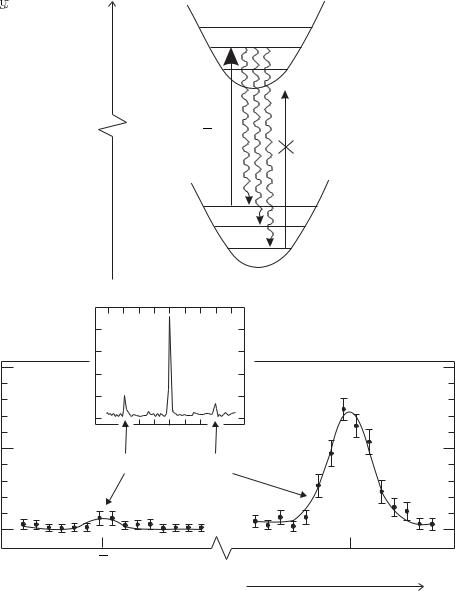
We have seen that typically Γ/2π is tens of MHz and ωv/2π 1 MHz. The vibrational energy levels have the same spacing ωv in both the ground and excited states of the ion since the vibrational frequency depends only on the charge-to-mass ratio of the ion and not its internal state, as illustrated in Fig. 12.10. The trapped ion absorbs light at the angular frequency of the narrow transition for a free ion ω0, and also at the frequencies ωL = ω0 ± ωv, ω0 ± 2ωv, ω0 ± 3ωv, etc. that correspond to transitions in which the vibrational motion of the ion changes. The vibrational levels in the ground and excited states are labelled by the vibrational quantum numbers v and v , respectively, and these sidebands correspond to transitions in which v = v. The energy of the bound system is reduced by using laser light at frequency ωL = ω0 − ωv to excite the first sideband of lower frequency, so that the ion goes into the vibrational level with v = v − 1 in the upper electronic state. This excited state decays back to the ground state—the most probable spontaneous transition is the one in which the vibrational level does not change so that, on average, the ion returns to the ground electronic state in a lower vibrational level than it started. A detailed explanation of the change in v during spontaneous emission would need to consider the overlap of the wavefunctions for the di erent vibrational levels and is not given here.33
This sideband cooling continues until the ion has been driven into the lowest vibrational energy level. An ion in the v = 0 level no longer absorbs radiation at ω0 − ωv, as indicated in Fig. 12.10—experiments use this to verify that the ion has reached this level by scanning the laser frequency to observe the sidebands on either side, as shown in Fig. 12.10(b); there is little signal at the frequency of the lower sideband, as predicted, but there is a strong signal at the frequency of the upper sideband.34 The lower sideband arises for the population in the v = 1 level (and any higher levels if populated), and the upper sideband comes from ions in v = 0 that make a transition to the v = 1 level. Thus the ratio of the signals on these two sidebands gives a direct measure of the
33The situation closely resembles that in the Franck–Condon principle that determines the change in vibrational levels in transitions between electronic states of molecules—the relevant potentials for an ion, shown in Fig. 12.10, are simpler than those for molecules.
34It is easy to be misled into thinking that the number of sidebands observed depends on the occupation of the vibrational levels of the trapped ion (especially if you are familiar with the vibrational structure of electronic transitions in molecules). This example shows that this is not the case for ions, i.e. sidebands arise for an ion that is predominantly in the lowest vibrational level. Conditions can also arise where there is very weak absorption at the frequencies of the sidebands, even though many vibrational levels are occupied, e.g. for transitions whose wavelength is much larger than the region in which the ions are confined. Although sidebands have been explained here in terms of vibrational levels, they are not a quantum phenomenon—there is an alternative classical explanation of sidebands in terms of a classical dipole that emits radiation while it is vibrating to and fro.
278 Ion traps
(a)
(b)
Signal (arbitrary units)
Frequency of laser radiation, 


Fig. 12.10 (a) The vibration levels of an ion in a harmonic trap have the same spacing for both the ground and excited electronic states. Excitation by light of frequency ωL = ω0 − ωv, followed by spontaneous emission, leads to a decrease in the vibrational quantum number, until the ion reaches the lowest level with v = 0, from whence there is no transition, as indicated by the dotted line at this frequency (but light at frequency ω0 and ω0 + ωv would excite the ion in v = 0). (b) The spectrum of a trapped ion shows sidebands on either side of the main transition. The inset figure shows the spectrum before sideband cooling. The enlarged part of the figure shows that after sideband cooling the signal on the upper sideband SU at angular frequency ω0 + ωv is stronger than the lower one SL at ω0 − ωv—this asymmetry indicates that the ion is mainly in the lowest vibrational state (i.e. vibrational quantum number much less than 1). The vertical axis gives the transition probability, or the probability of a quantum jump during the excitation of the narrow transition. After Diedrich et al. (1989). Part (b), copyright 1989 by the American Physical Society.
ratio of populations: in this example N (v = 1) /N (v = 0) = 0.05 so the ion spends most of its time in the lowest level. Thus the ion has almost the minimum energy attainable in this system.
Single ion experiments such as optical frequency standards with extremely high resolution (Section 12.6) do not need to cool the ion to the very lowest level—they just pick out the transition at ω0 from the wellresolved sidebands. The quantum computing experiments described in the next chapter, however, must have an initial state with all the ions in the lowest energy level of the trap (or very close to this ideal situation) to give complete control over the quantum state of the whole system. The preparation of all the trapped ions in the lowest vibrational level35 is complicated by the collective modes of vibration of a system with more than one trapped ion (Exercise 12.1), and the achievement of this initial state stretches the capability of laser cooling methods to their very limits.36
12.10Summary of ion traps
This chapter explored some of the diverse physics of ion trapping, ranging from the cooling of ions to temperatures of only 10−3 K in small ion traps to the production of highly-charged ions in the EBIT. Trapping of positrons was mentioned in Section 12.7.3 and ion traps make good containers for storing other types of antimatter such as antiprotons produced at particle accelerators.37 In recent experiments at CERN carried out by a large collaboration (Amoretti et al. 2002) these two antiparticles have been put together to produce anti-hydrogen. In the future it will be possible to do anti-atomic physics, e.g. to measure whether hydrogen and anti-hydrogen have the same spectra (a test of CPT invariance.) This high-energy trapping work has developed from accelerator-based experiments and probes similar physics.
At the opposite pole lies the work on the laser cooling of ions to extremely low energies. We have seen that the fundamental limit to the cooling of a bound system is quite di erent to the laser cooling of free atoms. Experimenters have developed powerful techniques to manipulate single ions and make frequency standards of extreme precision. The long decoherence times of trapped ions are now being exploited to carry out the manipulation of several trapped ions in experiments on quantum computation, which is the subject of the next chapter. Such experimental techniques give exquisite control over the state of the whole quantum system in a way that the founders of quantum mechanics could only dream about.
Further reading 279
35For neutral particles in magnetic traps, quantum statistics causes the atoms to undergo Bose–Einstein condensation into the ground state, even though they have a mean thermal energy greater than the spacing between trap energy levels. Quantum statistics does not a ect trapped ions because they are distinguishable—even if the ions are identical the mutual Coulomb repulsion keeps them far apart, as shown in Fig. 12.4, and the strong fluorescence enables the position of each ion to be determined.
36The alert reader may have noticed that we have not discussed the recoil limit, that plays such an important role for free particles. For sti traps the spacing of the vibrational energy levels greatly exceeds the recoil energy
ωv Erec, and the cooling limit of the trapped particle is determined by the zero-point energy.
37Just after its creation in high-energy collisions, the antimatter has an energy of MeV but it is moderated to energies of keV before trapping.
Further reading
The book on ion trapping by Ghosh (1995) gives a detailed account of these techniques. See also the tutorial articles by Wayne Itano (Itano et al. 1995) and David Wineland (Wineland et al. 1995), and the Nobel

280 Ion traps
38On the web site of the Nobel prizes. prize lecture of Wolfgang Paul.38 The National Physical Laboratory in the UK and the National Institute of Standards and Technology in the US provide internet resources on the latest developments and research.
Exercises
(12.1) The vibrational modes of trapped ions
Two calcium ions in a linear Paul trap lie in a line along the z-axis.
(a)The two end-cap electrodes along the z-axis
produce a d.c. potential as in eqn 12.23, with a2 = 106 V m−2. Calculate ωz .
(b)The displacements z1 and z2 of the two ions from the trap centre obey the equations
.. |
2 |
|
e2/4π 0 |
|
M z1 |
= −M ωz z1 |
− |
|
, |
(z2 − z1)2 |
||||
.. |
2 |
|
e2/4π 0 |
|
M z2 |
= −M ωz z2 |
+ |
|
. |
(z2 − z1)2 |
Justify the form of these equations and show that the centre of mass, zcm = (z1 + z2)/2 oscillates at ωz .
(c)Calculate the equilibrium separation a of two singly-charged ions.
(d)Find the frequency of small oscillations of the relative position z = z2 − z1 − a.
(e)Describe qualitatively the vibrational modes
of three ions in the trap, and the relative order of their three eigenfrequencies.39
(12.2) Paul trap
(a) For Hg+ ions in a linear Paul trap with dimensions r0 = 3 mm, calculate the maximum amplitude Vmax of the radio-frequency voltage at Ω = 2π × 10 MHz.
(b) For a√trap operating at a voltage V0 = Vmax/ 2, calculate the oscillation frequency of an Hg+ ion. What happens to a Ca+ ion when the electrodes have the same a.c. voltage?
(c) Estimate the depth of a Paul trap that has
√
V0 = Vmax/ 2, expressing your answer as a fraction of eV0.
(d)Explain why a Paul trap works for both positive and negative ions.
(12.3) Investigation of the Mathieu equation
Numerically solve the Mathieu equation and plot the solutions for some values of qx . Give examples of stable and unstable solutions. By trial and error, find the maximum value of qx that gives a stable solution, to a precision of two significant figures. Explain the di erence between precision and accuracy. [Hint. Use a computer package for solving di erential equations. The method in Exercise 4.10 does not work well when the solution has many oscillations because its numerical integration algorithm is too simple.]
(12.4) The frequencies in a Penning trap
A Penning trap confines ions along the axis by repulsion from the two end-cap electrodes; these have a d.c. positive voltage for positive ions that gives an axial oscillation frequency, as calculated in Exercise 12.1. This exercise looks at the radial motion in the z = 0 plane. The electrostatic potential in eqn 12.23 with a2 = 105 V m−2 leads to an electric field that points radially outwards, but the ion does not fly o in this direction because of a magnetic field of induction B = 1 T along the z-axis.
Consider a Ca+ ion.
(a)Calculate the cyclotron frequency.
(b)Find the magnetron frequency. [Hint. Work out the period of an orbit of radius r in a plane perpendicular to the z-axis by assuming a mean tangential velocity v = E(r)/B, where E(r) is the radial component of the electric field at r.]
39They resemble the vibrations of a linear molecule such as CO2, described in Appendix A; however, a quantitative treatment would have to take account of the Coulomb repulsion between all pairs of ions (not just nearest neighbours).
Exercises for Chapter 12 281
(12.5) Production of highly-charged ions in an EBIT
(a)Estimate the accelerating voltage required for
an electron beam voltage that produces hydrogenic silicon Si13+ in an EBIT.
(b)Calculate the radius of the first Bohr orbit (n = 1) in hydrogenic uranium, U+91.
(c)Calculate the binding energy of the electron in U+91 and express it as a fraction of the atom’s rest mass energy M c2.
(d)QED e ects contribute 3 × 10⁻⁵ eV to the
Web site:
http://www.physics.ox.ac.uk/users/foot
binding energy of the 1s ground configuration of atomic hydrogen. Express this as a fraction of the hydrogen atom’s rest mass. Estimate the magnitude of the QED contribution in the ground state of hydrogen-like uranium U+91 as a fraction of the rest mass. This fraction gives the precision ∆M/M with which the ion’s mass must be determined in order to measure QED e ects. Discuss the feasibility of doing this in an ion trap.
This site has answers to some of the exercises, corrections and other supplementary information.

13 |
Quantum computing |
|
13.1 |
Qubits and their |
|
|
properties |
283 |
13.2 |
A quantum logic gate |
287 |
13.3 |
Parallelism in quantum |
|
|
computing |
289 |
13.4 |
Summary of quantum |
|
|
computers |
291 |
13.5 |
Decoherence and |
|
|
quantum error |
|
|
correction |
291 |
13.6 |
Conclusion |
293 |
Further reading |
294 |
|
Exercises |
294 |
|
1Quantum computing requires precise control of the motion of the ions, i.e. their external degrees of freedom, as well as their internal state |F, MF .
Quantum computing will be a revolutionary new form of computation in the twenty-first century, able to solve problems inaccessible to classical computers. However, building a quantum computer is very di cult, and so far only simple logic gates have been demonstrated in experiments on ions in a linear Paul trap. The ideas of quantum computing have also been tested in experiments using nuclear magnetic resonance (NMR).
In the Paul trap, the ions sit in an ultra-high vacuum (pressure 10−11 mbar) so that collisions rarely happen, and the ions are well isolated from the environment. We have seen that these conditions enable extremely high-resolution spectroscopy of single ions because of the very small perturbations to the energy levels. Quantum computing requires more than one ion in the trap, and all of these ions must be cooled to the lowest vibrational level to give a well-defined initial quantum state for the system.1 This presents a much greater experimental challenge than the laser cooling of a single ion to reduce Doppler broadening, but it has been achieved in some experiments. The previous chapter describes the physics of the linear Paul trap but for the purposes of this chapter we simply assume that the trap produces a harmonic potential with strong confinement in the radial direction, so that the ions lie in a line along its z-axis, as shown in Fig. 13.1; their mutual electrostatic repulsion keeps the ions far enough apart for them to be seen separately.
Fig. 13.1 A string of four ions in a linear Paul trap. Coulomb repulsion keeps the ions apart and the gap corresponds to an ion in the dark state. In this experiment two laser beams simultaneously excite strong and weak transitions to give quantum jumps, as described in Section 12.6, so that each ion flashes on and o randomly. This snapshot of the system at a particular time could be taken to represent the binary number 1101. A quantum logic gate requires much more sophisticated techniques in which laser pulses determine precisely the initial state of each individual ion in the chain, as described in this chapter. Courtesy of Professors A. M. Steane and D. N. Stacey, D. M. Lucas and co-workers, Physics department, University of Oxford.

13.1 Qubits and their properties 283
13.1Qubits and their properties
A classical computer uses bits with two values 0 or 1 to represent binary numbers, but a quantum computer stores information as quantum bits or qubits (pronounced Q-bits). Each qubit has two states, labelled |0 and |1 in the Dirac ket notion for quantum states. Most theoretical discussions of quantum computing consider the qubit as a spin-1/2 object, so the two states correspond to spin down |ms = −1/2 and spin up |ms = +1/2 . However, for a trapped ion the two states usually correspond to two hyperfine levels of the ground configuration, as illustrated in Fig. 13.2. In the following discussion, |1 represents the ion in the upper hyperfine level and |0 is used for the lower hyperfine level, but all of the arguments apply equally well to spin-1/2 particles since the principles of quantum computing clearly do not depend on the things used as qubits. Ions, and other physical qubits, give a compact way of storing information, e.g. |1101 represents the binary number 1101 in Fig. 13.1, but the quantum features of this new way of encoding information only become apparent when we consider the properties of more than one qubit in Section 13.1.1. Even though a single qubit generally exists in a superposition of the two states, a qubit does not carry more classical information than a classical bit, as shown by the following argument. The superposition of the two states
ψqubit = a|0 + b|1 |
(13.1) |
obeys the normalisation condition |a|2 + |b|2 = 1 . We write this superposition in the general form
ψqubit = cos |
θ |
|
|0 + eiφ sin |
θ |
|1 eiφ . |
(13.2) |
|
|
|||||
2 |
2 |
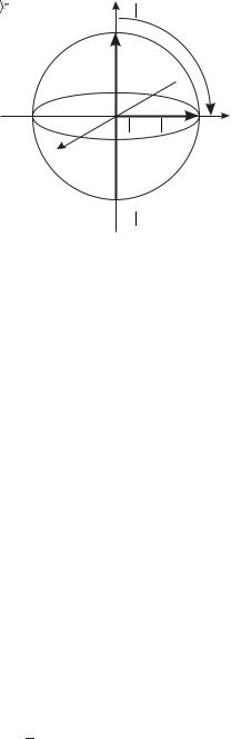
The overall phase factor has little significance and the possible states correspond to vectors of unit length with direction specified by two angles θ and φ. These are the position vectors of points lying on the surface of a sphere, as in Fig. 13.3. The state |0 lies at the north pole of this Bloch sphere and |1 at the south pole; all other position vectors are superpositions of these two basis states. Since these position vectors correspond to a simple classical object such as a pointer in three-dimensional space, it follows that the information encoded by each qubit can be modelled in a classical way.
The analogy between a qubit and a three-dimensional pointer seems to imply that a qubit stores more information than a bit with two possible values 0 or 1, e.g. like one of the hands of an analogue clock that gives us information about the time by its orientation in two-dimensional space. Generally, however, this is not true because we cannot determine the orientation of a quantum object as precisely as the hands on a clock. Measurements can only distinguish quantum states, with a high probability, if the states are very di erent from each other, occupying well-separated positions on opposite sides of the Bloch sphere. A measurement on a
Fig. 13.2 The two hyperfine levels in the ground state of an ion. Generally, experiments use an ion with total angular momentum J = 1/2 in the lowest electronic configuration, so that F = I ± 1/2. The qubits |0 and |1 correspond to two particular Zeeman
states in the two levels, e.g. |F, M and |F + 1, M , respectively.
284 Quantum computing
Fig. 13.3 The state |0 lies at the north pole of this Bloch sphere and |1 at the south pole; all other position vectors are superpositions of these two basis states. The Bloch sphere lies in the Hilbert space spanned by the two eigenvectors |0 and |1 . The Hadamard transformation defined in eqn 13.3 takes |0 → |0 + |1 (cf. Fig. 7.2).
2In this chapter wavefunctions are written without normalisation, which is the common convention in quantum computation.
spin-1/2 particle determines whether its orientation is up or down along a given axis. After that measurement the particle will be in one of those states since the act of measurement puts the system into an eigenstate of the corresponding operator. In the same way, a qubit will give either 0 or 1, and the read-out process destroys the superposition.
The Bloch sphere is very useful for describing how individual qubits transform under unitary operations. For example, the Hadamard transformation that occurs frequently in quantum computation (see the exercises at the end of this chapter) has the operator2
ˆ |
|0 + |1 , |
|
||
UH |0 → |
(13.3) |
|||
ˆ |
|
|
|
|
UH |1 → |0 − |1 . |
|
|||
This is equivalent to the matrix |
|
−1 . |
|
|
UˆH = √2 1 |
|
|||
1 |
|
1 |
1 |
|
The e ect of this unitary transformation of the state is illustrated in Fig. 13.3—it corresponds to a rotation in the Hilbert space containing the state vectors. This transformation changes |0 , at the north pole, into the superposition given in eqn 13.3 that lies on the equator of the sphere.
13.1.1Entanglement
We have already encountered some aspects of the non-intuitive behaviour of multi-particle quantum systems in the detailed description of the two
electrons in the helium atom (Chapter 3), where the antisymmetric spin
√
state [ |↓↑ − |↑↓ ]/ 2 corresponds to the wavefunction
Ψ = |01 − |10 |
(13.4) |
in the notation used in this chapter (without normalisation). This does not factorise into a product of single-particle wavefunctions:
Ψ = ψ1ψ2 , |
(13.5) |
13.1 Qubits and their properties 285
where
ψ1ψ2 = [ a|0 + b|1 ]1 [ c|0 + d|1 ]2 . |
(13.6) |
Here c and d are additional arbitrary constants, and the futility of attempting to determine these constants quickly becomes obvious if you try it. Generally, we do not bother with the subscript used to denote the particle, so |0 1|1 2 ≡ |01 and |1 1|1 2 ≡ |11 , etc. Multiple-particle systems that have wavefunctions such as eqn 13.4 that cannot be written as a product of single-particle wavefunctions are said to be entangled. This entanglement in systems with two, or more, particles leads to quantum properties of a completely di erent nature to those of a system of classical objects—this di erence is a crucial factor in quantum computing. Quantum computation uses qubits that are distinguishable, e.g. ions at well-localised positions along the axis of a linear Paul trap. We can label the two ions as Qubit 1 and Qubit 2 and know which one is which at any time. Even if they are identical, the ions remain distinguishable because they stay localised at certain positions in the trap. For a system of distinguishable quantum particles, any combination of the single-particle states is allowed in the wavefunction of the whole system:
Ψ = A|00 + B|01 + C|10 + D|11 . |
(13.7) |
The complex amplitudes A, B, C and D have arbitrary values. It is convenient to write down wavefunctions without normalisation, e.g.
Ψ = |00 + |01 + |10 + |11 , |
(13.8) |
Ψ = |00 + 2|01 + 3|11 , |
(13.9) |
Ψ = |01 + 5|10 . |
(13.10) |
Two of these three wavefunctions possess entanglement (see Exercise 13.1). We encounter examples with three qubits later (eqn 13.12).
In the discussion so far, entanglement appears as a mathematical property of multiple-particle wavefunctions, but what does it mean physically? It is always dangerous to ask such questions in quantum mechanics, but the following discussion shows how entanglement relates to correlations between the particles (qubits), thus emphasising that entanglement is a property of the system as a whole and not the individual particles. As a specific example consider two trapped ions. To measure their state, laser light excites a transition from state |1 (the upper hyperfine level) to a higher electronic level to give a strong fluorescence signal, so |1 is a ‘bright state’, while an ion in |0 remains dark.3 Wavefunctions such as those in eqns 13.4 and 13.10 that contain only the terms |10 and |01 always give one bright ion and the other dark, i.e. an anticorrelation where a measurement always finds the ions in di erent states. To be more precise, this corresponds to the following procedure. First, prepare two ions so that the system has a certain initial wavefunction Ψin, then make a measurement of the state of the ions by observing their fluorescence. Then reset the system to Ψin before another measurement. The record of the state of the ions for a sequence
3This is similar to the detection of quantum jumps in Section 12.6, but typically quantum computing experiments use a separate laser beam for each ion to detect them independently.