References

Добавил:

Upload Опубликованный материал нарушает ваши авторские права? Сообщите нам.

Вуз:

Национальный исследовательский университет «МИЭТ»

Предмет:

[НЕСОРТИРОВАННОЕ]

Файл:

Diss / 6 - 753p.pdf

Скачиваний:

Добавлен:

27.03.2016

Размер:

15.34 Mб

Скачать

☆

<<< < Предыдущая 37 38 39 40 41 42 43 44 45 46 47 4849 / 6849 50 51 52 53 54 55 56 57 58 59 60 61 > Следующая >>>

Kinetically Constrained Models

751

Furthermore proper modiﬁcations of the bisection-constrained technique also allow to deal with models which are reversible w.r.t. a high temperature Gibbs measure instead of μp [6] as well as models with long range constraints [7]. In both cases we establish positivity of the spectral gap in the whole ergodic region. The result for the long range models is particularly relevant since it allows, via proper renormalization and path techniques [7], to study the models with Kawasaki dynamics, namely the KCLG. In particular, by using the positivity of the spectral gap for a proper long range KCSM, we recently established [7] polynomial decay to equilibrium in inﬁnite volume as well as 1/L2 decay for the spectral gap on ﬁnite volume with boundary sources for the most popular KCLG, the so called Kob-Andersen model [21].

e−ρ(zk )eρ(w)

Z12 det(ωk (zl ))

1.M. Aizenman and J.L. Lebowitz, Metastability effects in bootstrap percolation. J. Phys. A 21(19), 3801–3813 (1988)

2.D. Aldous and P. Diaconis, The asymmetric one-dimensional constrained Ising model: Rigorous results. J. Stat. Phys. 107(5–6), 945–975 (2002)

3.L. Berthier, J.P. Garrahan, and S. Whitelam, Dynamic criticality in glass forming liquids. Phys. Rev. Lett. 92, 185705–185709 (2004)

4.L. Berthier, J.P. Garrahan, and S. Whitelam, Renormalization group study of a kinetically constrained model for strong glasses. Phys. Rev. E 71, 026128–026142 (2005)

5.S. Butler and P. Harrowell, The origin of glassy dynamics in the 2d facilitated kinetic Ising model. J. Chem. Phys. 83, 4454 (1991)

6.N. Cancrini, F. Martinelli, C. Roberto, and C. Toninelli, Facilitated spin models: Recent and new results. In: Koteczc, R. (ed.) Methods of Contemporary Mathetmatical Statistical Physics. Lecture Notes in Mathematics, vol. 1970, pp. 307–340. Springer, Berlin (2009)

7.N. Cancrini, F. Martinelli, C. Roberto, and C. Toninelli, Kinetically constrained lattice gases (2008)

8.N. Cancrini, F. Martinelli, C. Roberto, and C. Toninelli, Kinetically constrained spin models.

Probab. Theory Relat. Fields 140, 459–504 (2008)

9.P.G. De Benedetti and F.H. Stillinger, Supercooled liquids and the glass transition. Nature 410, 259–267 (2001)

10.S. Eisinger and J. Jackle, A hierarchically constrained kinetic Ising model. Z. Phys. B 84, 115–124 (1991)

11.M.R. Evans and P. Sollich, Glassy time-scale divergence and anomalous coarsening in a kinetically constrained spin chain. Phys. Rev. Lett. 83, 3238–3241 (1999)

12.G.H. Fredrickson, Recent developments in dynamical theories of the liquid glass transition. J. Chem. Phys. 39, 149–180 (1988)

13.G.H. Fredrickson and H.C. Andersen, Kinetic Ising model of the glass transition. Phys. Rev. Lett. 53, 1244–1247 (1984)

14.W. Gotze, Liquids, freezing and glass transition. In: Hansen et al., Les Houches Summer School Proceedings (1989)

15.I.S. Graham, M. Grant, and L. Piché, Model for dynamics of structural glasses. Phys. Rev. E 55, 2132–2144 (1997)

16.P. Harrowell, Visualizing the collective motion responsible for α and β relaxations in a model glass. Phys. Rev. E 48, 4359–4363 (1993)

17.A.E. Holroyd, Sharp metastability threshold for two-dimensional bootstrap percolation.

Probab. Theory Relat. Fields 125(2), 195–224 (2003)

752	Nicoletta Cancrini, Fabio Martinelli, Cyril Roberto and Cristina Toninelli

18.R.L. Jack, P. Mayer, and P. Sollich, Mappings between reaction-diffusion and kinetically constrained systems: A + A ↔ A and the FA model have upper critical dimension dc = 2. J. Stat. Mech. P03006 (2006)

19.J. Jackle, F. Mauch, and J. Reiter, Blocking transitions in lattice spin models with directed kinetic constraints. Physica A 184(3–4), 458–476 (1992)

20.T.R. Kirkpatrick, D. Thirumalai, and P. G Wolynes, Scaling concepts for the dynamics of viscous liquids near an ideal glassy state. Phys. Rev. A 40, 1045–1054 (1989)

21.W. Kob and H.C. Andersen, Kinetic lattice-gas model of cage effects in high-density liquids and a test of mode-coupling theory of the ideal-glass transition. Phys. Rev. E 48, 4359–4363 (1993)

22.G. Kordzakhia and S. Lalley, Ergodicity and mixing properties of the northeast models. J. Appl. Probab. 43(3), 782–792 (2006)

23.J. Reiter, Statics and dynamics of the 2-spin-facilitated kinetic Ising-model. J. Chem. Phys. 95(1), 544–554 (1991)

24.F. Ritort and P. Sollich, Glassy dynamics of kinetically constrained models. Adv. Phys. 52(4), 219–342 (2003)

25.C. Toninelli and G. Biroli, A new class of cellular automata with a discontinuous glass transition. J. Stat. Phys. 130, 83–112 (2008)

26.C. Toninelli, G. Biroli, and D.S. Fisher, Spatial structures and dynamics of kinetically constrained models for glasses. Phys. Rev. Lett. 92(1–2), 185504 (2004)

27.E.R. Weeks, J.C. Crocker, A.C. Levitt, A. Schoﬁeld, and D.A. Weitz, Three-dimensional direct imaging of structural relaxation near the colloidal glass transition. Science 287, 627–631 (2000)

The Distributions of Random Matrix Theory and their Applications

Craig A. Tracy and Harold Widom

Abstract This paper surveys the largest eigenvalue distributions appearing in random matrix theory and their application to multivariate statistical analysis.

1 Random Matrix Models: Gaussian Ensembles

A random matrix model (RMM) is a probability space (Ω, P, F ) where the sample space Ω is a set of matrices. There are three classic ﬁnite-N RMM called the Gaussian ensembles (see, e.g. [23] and for early history [30]):

•Gaussian Orthogonal Ensemble (GOE, β = 1)

–Ω = N × N real symmetric matrices

–P = unique (up to a choice of the mean and variance) measure that is invariant under orthogonal transformations and the algebraically independent matrix elements are i.i.d. random variables. Explicitly (for mean zero and a choice of the variance), the density is

cN exp − tr(A2)/2 dA,				(1)
where cN is a normalization constant and dA	=	dAii	i<j	dAij , the prod-
	=	i	i<j

uct Lebesgue measure on the algebraically independent matrix elements.

• Gaussian Unitary Ensemble (GUE, β = 2)

Craig A. Tracy

Department of Mathematics, University of California, Davis, CA 95616, USA, e-mail: tracy@math.ucdavis.edu

Harold Widom

Department of Mathematics, University of California, Santa Cruz, CA 95064, USA, e-mail: widom@ucsc.edu

This work was supported by the National Science Foundation under grants DMS-0553379 (ﬁrst author) and DMS-0552388 (second author).

V. Sidoraviciusˇ (ed.), New Trends in Mathematical Physics,	753
© Springer Science + Business Media B.V. 2009

λmax

754	Craig A. Tracy and Harold Widom

–Ω = N × N hermitian matrices

–P = unique measure (again up to a choice of the mean and variance) that is invariant under unitary transformations and the algebraically independent real

and imaginary matrix elements are i.i.d. random variables. Again the density is of the form (1) with dA = i dAii i<j d Re(Aij ) d Im(Aij ).

•Gaussian Symplectic Ensemble (GSE, β = 4) (see [23] for a deﬁnition)

For A in any of the above Gaussian ensembles, let λ1(A) ≤ · · · ≤ λN (A) := denote the eigenvalues of A. These eigenvalues are real and deﬁne random variables on the respective probability spaces. (With probability one the eigenvalues are distinct.) Since these Gaussian ensembles are deﬁned by invariant measures, one can explicitly compute the joint distribution of eigenvalues and show that it has the

following density with respect to Lebesgue measure:

Pβ,N (x1, . . . , xN ) = CN ,β		N
Pβ,N (x1, . . . , xN ) = CN ,β	\|xi − xj \|β e−βxi2/2, β = 1, 2, 4,
	1≤i<j ≤N	i=1

where CN ,β is a known normalization constant [23]. The form of the joint density explains the usefulness of the β notation.

1.1Largest Eigenvalue Distributions Fβ .

Painlevé II Representations

Generally speaking, the interest lies in limit laws as N → ∞. As is familiar from the central limit theorem, to get nontrivial limits one must center and normalize the random variables. Here the main focus is on the limit law associated with the largest

eigenvalue. If

FN ,β (t ) := Pβ,N (λmax < t ) , β = 1, 2, 4,

denotes the distribution function of the largest eigenvalue, then the basic limit laws [37–39] state that1

	√		σ x
	√	N +	σ x
Fβ (x) := Nlim FN ,β 2σ		N +	N 1/6	, β = 1, 2, 4,
→∞
exist and are given explicitly by
F2(x) = exp − x ∞(y − x)q2(y) dy					(2)

1 Here σ is the standard deviation of the Gaussian distribution on the off-diagonal matrix ele-

√

ments. For the normalization we’ve chosen, σ = 1/ 2; however, other choices are common.

The Distributions of Random Matrix Theory and their Applications

755

where q is the unique solution2 to the Painlevé II equation

d2q = xq + 2q3

dx2

satisfying the boundary condition3

q(x) Ai(x)

as x → ∞.

(3)

It is known [17] that

q(x) =

−

1 +

+ O

as x → −∞.

The orthogonal and symplectic distributions [39] are

∞

1/2

F1(x) = exp

−

q(y) dy

(F2(x))

∞

F4(x/√

) = cosh

q(y) dy

(F2(x))1/2 .

Graphs of the densities fβ := dFβ /dx are in Fig. 1 and some statistics of Fβ be found in the Table 1.

(4)

(5)

can

Fig. 1 Largest eigenvalue densities fβ (x) = dFβ /dx, β = 1, 2, 4 where Fβ are deﬁned in (2), (4) and (5)

2That such a unique solution exists is a nontrivial fact ﬁrst proved by Hastings and McLeod [17]; and for this reason, q is often called the Hastings-McLeod solution. See [15] for a detailed account of Painlevé transcendents.

3Ai is the Airy function.

756	Craig A. Tracy and Harold Widom

1.1.1 Tail behavior of Fβ

The asymptotics for Fβ (x) as x → +∞ follows straightforwardly from (2)–(5). To state the results it is ﬁrst convenient to introduce

		1	∞	2
F (x) = exp	−			(y − x)q(y)	dy ,
F (x) = exp	−	2	x	(y − x)q(y)	dy ,
		1	∞
E(x) = exp	−			q(y) dy
E(x) = exp	−	2	x	q(y) dy

so that

(x) = E(x)F (x), F2(x) = F (x)2, and

√

(x/

2) =

E(x) + E(x)

F (x).

Then as x → +∞

e− 43 x3/2

F (x) = 1 −

1 + O

x3/2

32π x3/2

E(x) = 1 −

e− 32 x3/2

4√

x3/2

1 + O

x3/2

from which the asymptotics for Fβ follows.

The asymptotics as x → −∞ are much more difﬁcult and the complete solution was only recently achieved for β = 1, 2, 4 [4]. We quote the ﬁnal results and refer the reader to [4] for a history of this problem. As x → −∞

3/2

e−

|x| −

3√

|x|

F1(x) =

1 −

√

+ O |x|−3

τ1

x 1/16

3/2

2 x

e−

|x|3

F2(x) =

τ2

1 +

+ O |x|−6

x 1/8

3/2

e−

|x| +

3√

|x|

F4(x/√2) =

τ4

1 +

√

+ O |x|−3

x 1/16

3/2

2 x

where

τ1 = 2−11/48e 21 ζ (−1),

τ2 = 21/24eζ (−1),

τ4 = 2−35/48e 21 ζ (−1)

and ζ (−1) = −0.1654211437 . . . is the derivative of the Riemann zeta function evaluated at −1.

The Distributions of Random Matrix Theory and their Applications

757

1.1.2 Numerical evaluation of Fβ

Particularly for applications to data analysis, it is useful to have numerical evaluations of the distributions Fβ . Chapter 7 of Dieng’s Ph.D. thesis [12] gives MATLABTM code to evaluate and plot these distributions. Tables of the HastingsMcLeod solution to Painlevé II and F1,2 can be found on Prähofer’s homepage [31].4 A different approach [6] to the numerical evaluation of Fβ is based on the Fredholm determinant representations for Fβ (see, e.g. [40]).

Table 1 The mean (μβ ), variance (σβ2), skewness (Sβ ) and kurtosis (Kβ ) of Fβ . The high-precision numbers are courtesy of Michael Prähofer and Folkmar Bornemann

β	μβ	σ 2	Sβ	Kβ
		β
1	−1.206 533 574	1.607 781 034	0.293 464 524	0.165 242 938
2	−1.771 086 807	0.813 194 792	0.224 084 203	0.093 448 087
4	−2.306 884 893	0.517 723 721	0.165 509 494	0.049 195 157

1.2 Next-Largest, Next-Next Largest, Etc. Eigenvalue Distributions

There exist Painlevé II type representations for the limiting distributions of the nextlargest eigenvalue (λN −1), next-next largest eigenvalue (λN −2), etc. The unitary case was examined some time ago [38] but only recently did Dieng [11] derive limiting distributions for the orthogonal and symplectic cases. It should be remarked that the results in the orthogonal case were somewhat surprising. Figure 2 displays simulations for the four largest eigenvalues of N = 1000 GOE matrices and their respective limiting distributions.

2 Universality Theorems

A natural question is to what extent do the above limit laws depend upon the Gaussian and invariance assumptions for the probability measure?

2.1 Invariant Ensembles

A more general class of invariant RMM results by replacing the Gaussian measures with

4 Note that the Hastings-McLeod solution in the Prähofer tables is denoted u(s) and in the notation here u(s) = −q(s).

14 A4 −

758	Craig A. Tracy and Harold Widom

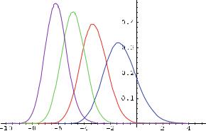
Fig. 2 A histogram of the four largest (centered and normalized) eigenvalues for 104 realizations of 103 × 103 GOE matrices. Solid curves are the limiting distributions from [11]. Figure a courtesy of Momar Dieng

dPN (A) = cN ,β exp (−β tr(V (A))/2) dA

where V is a polynomial of even degree and positive leading coefﬁcient. This implies that the joint density for the eigenvalues is

Pβ,V ,N (x1, . . . , xN ) = CV ,N ,β		N
Pβ,V ,N (x1, . . . , xN ) = CV ,N ,β	\|xi − xj \|β e−βV (xi )/2, β = 1, 2, 4,
	1≤i<j ≤N	i=1

(6)

where CV ,N ,β is a normalization constant [23]. Unitary ensembles (β = 2) are technically simpler than the orthogonal and symplectic ensembles (β = 1, 4), but both require for general V powerful Riemann-Hilbert methods [9] for the asymptotic analysis. The main conclusions from these studies for the limiting distribution of the largest eigenvalue are

Theorem 1. There exist constants zN(β) and sN(β) such that

	P	λmax − zN(β)
Nlim	β,V ,N		(β)	≤ t = Fβ (t ), β = 1, 2, 4,
→∞			sN

where the Fβ are given by (2), (4) and (5).

The results for the unitary case (β = 2) are due to Deift, Kriecherbaur, McLaughlin, Venakides and Zhou [10] and the orthogonal/symplectic results are recent work of Deift and Gioev [8]. The universality theorem for special case V (A) =

gA2 is due to Bleher and Its [5] (β = 2) and Stojanovic [36] (β = 1). These deep theorems broadly extend the domain of attraction of the Fβ limit laws. Deift’s ICM 2006 lecture [7] is a recommended overview for these developments.

The Distributions of Random Matrix Theory and their Applications

759

2.2 Wigner Ensembles

Wigner matrices are RMM of complex hermitian or real symmetric N × N matrices H

1
H = √N (Aij )i,jN	=1

where Aij , 1 ≤ i < j ≤ N are i.i.d. complex or real random variables with distribution μ. The diagonal matrix elements are i.i.d. real random variables independent of the off-diagonal elements. The diagonal probability distribution is centered, independent of N and has ﬁnite variance. They are called Wigner matrices since Wigner in 1955 ﬁrst studied the limiting distribution of the empirical spectral measure under the assumption that μ has ﬁnite variance. The limiting spectral measure is the famous Wigner semicircle distribution. We denote the Wigner measure on the space of either complex Hermitian or real symmetric N × N matrices by PW,N

Except in the case of the Gaussian distribution, the Wigner ensembles deﬁne noninvariant measures. For this reason no explicit formulas for the joint distribution of eigenvalues, such as (6) for invariant measures, are known. Thus the techniques used to prove universality theorems have a completely different ﬂavor.

Soshnikov [33] proved, under the additional assumptions that μ is symmetric (all odd moments are zero) and the distribution decays as at least as fast as a Gaussian distribution together with a normalization on the variances,5 the following universality statement for the largest eigenvalue λmax of Wigner random matrices

Theorem 2.	P		x
Nlim	P		x
Nlim	W,N	λmax ≤ 1 +	2N 2/3	= Fβ (x)
→∞

with β = 1 for real symmetric matrices and β = 2 for complex hermitian matrices.

The importance of Soshnikov’s theorem is the universality of Fβ has been established for ensembles for which the “integrable” techniques, e.g. Fredholm theory, Riemann-Hilbert methods, Painlevé theory, are not directly applicable. Current research [29] is exploring the relaxation of the symmetry constraint on the underlying distribution μ.

3 Multivariate Statistical Analysis

As Johnstone [22] remarked:

It is a striking feature of the classical theory of multivariate statistical analysis that most of the standard techniques—principal components, canonical correlations, multivariate analysis of variance (MANOVA), discriminant analysis and so forth—are founded on the eigenanalysis of covariance matrices.

5 For real symmetric matrices the normalization is EW,N (Hij2 ) = 41 ,	1 ≤ i < j ≤ N and for
complex hermitian matrices EW,N (Re(Hij )2) = EW,N (Im(Hij )2) = 81 .

760	Craig A. Tracy and Harold Widom

Thus it is not surprising that the methods of random matrix theory have important applications to multivariate statistical analysis. We now survey some of these recent developments drawing heavily on Johnstone’s 2006 ICM lecture [21]. We have also beneﬁted from the unpublished survey by Péché [28].

3.1 Principal Component Analysis (PCA)

Recall that in PCA with p variables one distinguishes between the population eigenvalues j , which are the eigenvalues of the underlying p × p covariance matrix

Σ = (Cov(Xk , Xk ))1≤k,k ≤p ,

and the sample eigenvalues ˆ , which are the (random) eigenvalues of the sample

covariance matrix

S= 1 XXT . n

Here X is the p × n data matrix and n is the number of observations of the p variables. (A column of X represents one observation of the p variables.) Since the parameters of the underlying probability model describing the random variables X1, . . . , Xp are unknown, the problem is to deduce properties of Σ from the observed sample covariance matrix S.

The simplest model is to assume X = (X1, . . . , Xp ) is a p-variate Gaussian distribution Np (μ, Σ ) and the data matrix X is formed by n independent draws X1, . . . , Xn. (For simplicity we consider μ = 0.) The p × p matrix A = XXT is said to have p-variate Wishart distribution on n degrees of freedom, Wp (n, Σ ). We

denote the eigenvalues of A by l1	≥	l	2 ≥ · · · lp ≥ 0 (so lj	= n ˆj ). The joint dis-
		l

tribution of the eigenvalues lj has been known for some time (e.g. Muirhead [24], Theorem 3.2.18) and is complicated by the fact it involves an integral over the orthogonal group O(p).

3.2 Testing the Null Hypothesis

The null hypothesis H0 is the statement that there are no correlations amongst the p variables, i.e. Σ = I . Under H0 all the population eigenvalues equal one, but as

been known for some time6 there is a “spread” in the sample eigenvalues ˆ . To

j assess whether “large” observed eigenvalues justify rejecting the null hypothesis, we need an approximation to the null hypothesis distribution of the largest sample eigenvalue,

6 For Σ = I , the density of eigenvalues of S follows the Marchenko-Pastur distribution, a generalization of the Wigner semicircle distribution.

The Distributions of Random Matrix Theory and their Applications										761
P		> t	\|	H	0	=	W	p	(n, I ) .	(7)
	ˆ1		\|		0	=		p

This approximation is provided by the following theorem of Johnstone [20].

Theorem 3.

P			μ		σ		x H		F	(x)
		≤		np +		np		→
	n ˆ1						\| 0		1

where the limit is n → ∞, p → ∞ such that p/n → γ (0, ∞), F1 is the largest eigenvalue distribution (4), and the centering and norming constants are

										2
				1					1	2
μnp =		n −				+	p −				,				(8)
μnp =		n −		2		+	p −		2		,				(8)
σnp = √			+ √					1			+	1		1/3	(9)
	n				p			1				1		.

								n −		1		p −	1
								n −		2		p −	2

Several remarks are in order.

1.The appearance of the fractions 12 in μnp and σnp appear to improve the rate of convergence to F1 to “second-order accuracy” [21]. With this choice of constants, F1 provides a good approximation for rather small values of p. (See Johnstone’s comparisons with the tables of Chen [21].)

2.El Karoui [14] shows the theorem holds more generally as

p/n → γ [0, ∞].

3.For complex data matrices with Σ = I , there are corresponding limit theorems where now convergence is to F2 [18, 20].

4.Soshnikov [34] and Péché [27] have removed the assumption of Gaussian samples. They assume that the matrix elements Xij of the data matrix X are independent random variables with a common symmetric distribution whose moments grow not faster than the Gaussian ones. We refer the reader to [27] for a description of the centering and norming constants. Limit theorems for complex data matrices are also proved.

5.To summarize, given the centering and norming constants (8) and (9) together with tables such as Table 2, one has a good approximation to the null distribution function (7).

3.3 Spiked Populations: BBP Phase Transition

As mentioned above, an essential difﬁculty in extending the above limit laws for

ˆ1	when the A	=	XXT		p	(n, Σ ), Σ	=	I , is the presence of a certain integral
	when the A		XXT		W	(n, Σ ), Σ		I , is the presence of a certain integral

over the orthogonal group O(p) in the joint distribution of eigenvalues of A. In the case of complex Wishart matrices, the corresponding integral in the joint distribution

762		Craig A. Tracy and Harold Widom
Table 2 Values of x for given P(χ1 ≥ x) where χ1 has distribution F1
	x	P(χ1 ≥ x)
	2.02345	0.01
1.59776		0.02
1.33321		0.03
1.13706		0.04
0.97931		0.05
0.84633		0.06
0.73069		0.07
0.62792		0.08
0.53508		0.09
0.45014		0.10

of eigenvalues is over the unitary group U(p) which, fortunately, can be explicitly evaluated by use of the Harish-Chandra-Itzykson-Zuber formula, see, e.g. [41].

We now describe the limit theorem of Baik, Ben Arous and Péché [3] where they consider the complex Wishart ensemble with the p × p covariance matrix

Σ = diag ( 1, . . . , r , 1, . . . , 1) .

For ease of exposition of their results, we consider r = 1 with 1 > 1. As before we consider the limit

p → ∞,

n → ∞ such that

→ γ

≥ 1.

(10)

Deﬁne

wc = 1 + √

Theorem 4.

With

as above (r =

1), let

ˆ1 denote the largest eigenvalue of the

sample covariance matrix.

• If 1 ≤ 1 < wc , then in the limit (10)

n2/3

≤ x

→ F2(x),

ˆ1 − μ

where F2 is given by (2) and

μ = (1 + √

1/3

)2,

σ = (1 + √

) 1 + √

• If π1 > wc , then in the limit (10)

n1/2

− μ1)

≤ x

→ Φ(x),

σ1

ˆ1

where Φ is the standard normal distribution and

The Distributions of Random Matrix Theory and their Applications

763

	γ		2		γ
μ1 = 1 1 +		,	σ1 = 1	1 −		.
	1 − 1				( 1 − 1)2

Remarks:

1.The BBP theorem “shows that a single eigenvalue of the true covariance Σ may drastically change the limiting behavior of the largest eigenvalue of sample covariance matrices. One should understand the above result as the statement that the eigenvalues exiting the support of the Marchenko-Pastur distribution form a small bulk of eigenvalues. This small bulk exhibits the same eigenvalue statistics as the eigenvalues of a non-normalized GUE (resp. GOE) matrix” [28].

2.If π1 = wc the limiting distribution is a generalization of F2 expressible in terms

3.	of the same Painlevé II function q [1].		c	is simple, then	ˆ1
3.	For real Wishart matrices, Paul [26] shows that if π1	> w	c	is simple, then	ˆ1
		> w
	exhibits Gaussian ﬂuctuations.
4.	El Karoui [13] ﬁnds a large class of complex Wishart matrices Wp (Σ, n) which
	have a F2 limit law for ˆ1.

5.Patterson, Price and Reich [25] have applied these results to problems of population structure arising from genetic data. See Harding [16] for an application in economics.

4 Conclusions

In this note we have surveyed some basic properties of the largest eigenvalue distributions Fβ , their appearance as limit laws for large classes of random matrix models as well as their application to principal component analysis. We mention that these same distributions play an analogous role in canonical correlations [22] as they do in PCA.

We have not discussed the appearance of the Fβ limit laws in growth processes. This line of research began with Baik, Deift & Johansson’s work [2] on Ulam’s Problem of the length of the longest increasing subsequence of a random permutation. (See also Johansson [18, 19] as well as [35] for a recent review.) Nor have we discussed the generalization of Fβ to all real β > 0 by Ramírez, Rider and Virág [32].

References

1.J. Baik, Painlevé formulas of the limiting distributions for nonnull complex sample covariance matrices of spiked population models. Duke Math. J. 133, 205–235 (2006)

2.J. Baik, P. Deift, and K. Johansson, On the distribution of the length of the longest increasing subsequence of random permutations. J. Am. Math. Soc. 12, 1119–1178 (1999)

3.J. Baik, G. Ben Arous, and S. Péché, Phase transition of the largest eigenvalue for non-null complex sample covariance matrices. Ann. Probab. 33, 1643–1697 (2005)

764	Craig A. Tracy and Harold Widom

4.J. Baik, R. Buckingham, and J. DiFranco, Asymptotics of the Tracy-Widom distributions and the total integral of a Painlevé II function. Commun. Math. Phys. 280, 463–497 (2008)

5.P. Bleher and A. Its, Semiclassical asymptotics of orthogonal polynomials, Riemann-Hilbert problem, and universality in the matrix model. Ann. Math. 150, 185–266 (1999)

6.F. Bornemann, On the numerical evaluation of Fredholm determinants. arXiv:0804.2543

7.P. Deift, Universality for mathematical and physical systems, International Congress of Mathematicians, vol. I, pp. 125–152, Eur. Math. Soc., Zürich (2007). Available in preprint form at http://front.math.ucdavis.edu/0603.4738

8.P. Deift and D. Gioev, Universality at the edge of the spectrum for unitary, orthogonal, and symplectic ensembles of random matrices. Commun. Pure Appl. Math. 60, 867–910 (2007)

9.P.A. Deift and X. Zhou, A steepest descent method for oscillatory Riemann-Hilbert problems. Asymptotics for the MKdV equation. Ann. Math. 137, 295–368 (1993)

10.P. Deift, T. Kriecherbauer, K.T.-R. McLauglin, S. Venakides, and X. Zhou, Uniform asymptotics for polynomials orthogonal with respect to varying exponential weight and applications to universality questions in random matrix theory. Commun. Pure Appl. Math. 52, 1335–1425 (1999)

11.M. Dieng, Distribution functions for edge eigenvalues in orthogonal and symplectic ensembles: Painlevé representations. Int. Math. Res. Not. 37, 2263–2287 (2005)

12.M. Dieng, Distribution functions for edge eigenvalues in orthogonal and symplectic ensembles: Painlevé Representations II. arXiv:math/0506586

13.N. El Karoui, Tracy-Widom limit for the largest eigenvalue of a large class of complex sample covariance matrices. Ann. Probab. 35, 663–714 (2007)

14.N. El Karoui, On the largest eigenvalue of Wishart matrices with identity covariance when n, p and p/n tend to inﬁnity. arXiv:math/0309355

15.A.S. Fokas, A.R. Its, A.A. Kapaev, and V.Yu. Novokshenov, Painlevé Transcendents: The Riemann-Hilbert Approach. American Mathematical Society, Providence (2006)

16.M. Harding, Explaining the single factor bias of arbitrage pricing models in ﬁnite samples. Econ. Lett. 99, 85–88 (2008)

17.S.P. Hastings and J.B. McLeod, A boundary value problem associated with the second Painlevé transcendent and the Korteweg-de Vries equation. Arch. Ration. Mech. Anal. 73, 31–51 (1980)

18.K. Johansson, Shape ﬂuctuations and random matrices. Commun. Math. Phys. 209, 437–476 (2000)

19.K. Johansson, Toeplitz determinants, random growth and determinantal processes. ICM 2002, vol. III, pp. 53–62

20.I. Johnstone, On the distribution of the largest principal component. Ann. Stat. 29, 295–327 (2001)

21.I. Johnstone, High dimensional statistical inference and random matrices. International Congress of Mathematicians, vol. I, pp. 307–333, Eur. Math. Soc. Zürich (2007). Available in preprint form at http://front.math.ucdavis.edu/0611.5589

22.I. Johnstone, Multivariate analysis and Jacobi ensembles: Largest eigenvalue, Tracy-Widom limits and rates of convergence. Preprint arXiv:0803.3408

23.M.L. Mehta, Random Matrices, 2nd edn. Academic Press, Dordrecht (1991)

24.R.J. Muirhead, Aspects of Multivariate Statistical Theory. Wiley, New York (1982)

25.N. Patterson, A.L. Price, and D. Reich, Population structure and eigenanalysis. PLoS Genet. 2(12), e190 (2006)

26.D. Paul, Asymptotics of the leading sample eigenvalues for a spiked covariance model. Stat. Sin. 17, 1617–1642 (2007)

27.S. Péché, Universality results for largest eigenvalues of some sample covariance matrices. arXiv:0705.1701

28.S. Péché, The edge of the spectrum of random matrices. Habilitation à diriger des recherches. Université Joseph Fourier Grenoble I (to be submitted)

29.S. Péché and A. Soshnikov, On the lower bound of the spectral norm of symmetric random matrices with independent entries. Elect. Commun. Probab. 13, 280–290 (2008)

The Distributions of Random Matrix Theory and their Applications

765

30.C.E. Porter, Statistical Theories of Spectra: Fluctuations. Academic Press, Dordrecht (1965)

31.M. Prähofer, http://www-m5.ma.tum.de/pers/praehofer/

32.J.A. Ramírez, B. Rider, and B. Virág, Beta ensembles, stochastic Airy spectrum, and a diffusion. arXiv:math.PR/0607331

33.A. Soshnikov, Universality at the edge of the spectrum in Wigner random matrices. Commun. Math. Phys. 207, 697–733 (1999)

34.A. Soshnikov, A note on universality of the distribution of the largest eigenvalue in certain classes of sample covariance matrices. J. Stat. Phys. 108, 1033–1056 (2002)

35.H. Spohn, Exact solutions for KPZ-type growth processes, random matrices, and equilibrium shapes of crystals. Physica A 369, 71–99 (2006)

36.A. Stojanovic, Universality in orthogonal and symplectic invariant matrix models with quartic potential. Math. Phys., Anal. Geom. 3, 339–373 (2000)

37.C.A. Tracy and H. Widom, Level-spacing distribution and the Airy kernel. Phys. Lett. B 305, 115–118 (1993)

38.C.A. Tracy and H. Widom, Level-spacing distribution and the Airy kernel. Commun. Math. Phys. 159, 151–174 (1994)

39.C.A. Tracy and H. Widom, On orthogonal and symplectic matrix ensembles. Commun. Math. Phys. 177, 727–754 (1996)

40.C.A. Tracy and H. Widom, Matrix kernels for the Gaussian orthogonal and symplectic ensembles. Ann. Inst. Fourier, Grenoble 55, 2197–2207 (2005)

41.P. Zinn-Justin and J.-B. Zuber, On some integrals over the U(N ) unitary group and their large N limit. J. Phys. A, Math. Gen. 36, 3173–3193 (2003)

Hybrid Formalism and Topological Amplitudes

Jürg Käppeli, Stefan Theisen, and Pierre Vanhove

Abstract We study four-dimensional compactiﬁcations of type II superstrings on Calabi-Yau spaces in the hybrid formalism. Chiral and twisted-chiral interactions are rederived, which involve the coupling of the compactiﬁcation moduli to two powers of the Weyl-tensor and of the derivative of the universal tensor ﬁeld-strength. We review the formalism and provide details of some of its technicalities.

1 Introduction

Type II string compactiﬁed on a Calabi–Yau 3-fold gives rise to N = 2 supergravity in four dimension. Most calculations of string scattering amplitudes, and therefore of the construction of the low-energy-effective action, are based on the Ramond-Neveu-Schwarz (RNS) formulation of the superstring. A drawback of this formulation is that spacetime supersymmetry is not manifest and is achieved only after GSO projection.

An alternative formulation without these complications is the hybrid formulation. Hybrid string theory can be obtained by a ﬁeld redeﬁnition from the gaugeﬁxed RNS string or by covariantizing the Green-Schwarz (GS) string in light-cone gauge. In this sense, worldsheet reparametrizations are gauge-ﬁxed in the hybrid formulation. Nevertheless, there is no need for ghost-like ﬁelds in the formalism since the theory can be formulated as a N = 4 topological theory and amplitudes

Jürg Käppeli

Institut für Physik, Humboldt Universität, Berlin, Germany, e-mail: kaeppeli@aei.mpg.de

Stefan Theisen

Max-Planck-Institut für Gravitationsphysik, Albert-Einstein-Institut, Golm, Germany, e-mail: theisen@aei.mpg.de

Pierre Vanhove

CEA/DSM/SPhT, URA au CNRS, CEA/Saclay, 91191 Gif-sur-Yvette, France, e-mail: pierre.vanhove@cea.fr

V. Sidoraviciusˇ (ed.), New Trends in Mathematical Physics,	767
© Springer Science + Business Media B.V. 2009

768	Jürg Käppeli, Stefan Theisen, and Pierre Vanhove

can be computed directly by the methods of topological string theory [12]. The theory consists of two completely decoupled twisted worldsheet SCFT, one describing the spacetime part, one the internal part. Despite being twisted, hybrid string theory describes the full theory, i.e., it computes also non-topological amplitudes. Hybrid type IIA and IIB string theories are distinguished by the relative twisting of the leftand right-moving sector of the internal SCFT. When working with either type one is therefore committed to a given ﬁxed twisting.

The hybrid formulation was developed in a series of papers by N. Berkovits and various collaborators [12, 7, 10]. It was reviewed in [9]. One purpose of this note is our attempt to ﬁll in details of some of the more technical aspects. This is done in Sect. 2 and the Appendices B and C, the content of which is well known to the few experts in the ﬁeld, but often not readily accessible.

The main application of hybrid strings in this note are presented in Sects. 3 and 4. We extend the analysis of higher order derivative interactions to the twisted-chiral sector. The procedure is analogous to the computation in the chiral sector given [12]. Even though one is working with a ﬁxed relative twisting, giving rise to either type IIA or type IIB, it is shown that the chiral and twisted-chiral couplings of each type II theory depend on both the A-model and B-model topological partition functions. In the effective action these amplitudes give rise to couplings of compactiﬁcation moduli to two powers of the Weyl tensor or of the derivative of the universal tensor ﬁeld-strength. In the RNS formulation these couplings were discussed in [4].

Another possible application is ﬂux compactiﬁcations of the type II string with N = 1 spacetime supersymmetry. The breaking N = 2 → N = 1 results from auxiliary ﬁelds acquiring vacuum expectation values [30]. Due to its manifest spacetime supersymmetry, the hybrid formulation might be the most suitable. First steps in this direction were already taken in [24, 26].

2 Compactiﬁed String Theory in RNS and Hybrid Variables

In this section we present a detailed account of the ﬁeld mapping between the variables of the Ramond-Neveu-Schwarz (RNS) formulation of those of the hybrid formulation of the superstring. We consider here only Calabi-Yau compactiﬁcations to four spacetime dimensions and split all variables into a spacetime and an internal part. The internal part is practically the same for the RNS and the hybrid formulation, while the two descriptions of the spacetime are different.

2.1 Hybrid Variables

Type II and heterotic string theory compactiﬁed on a Calabi-Yau three-fold can be formulated within a covariant version of the Green-Schwarz (GS) formulation [7, 10]. The spacetime part consists of four bosons xm, two pairs of left-moving canon-

+ c ¯ ¯ +

p,θ

Hybrid Formalism and Topological Amplitudes		¯β		769
ically conjugate Weyl fermions (pα , θ β ) and	¯	¯β		), both of conformal weight
	¯		˙
	(pα˙	, θ

(1, 0) and a chiral boson ρ with action

¯ ¯

+ ˜

∂x

∂xm

p ∂θα

+ ¯

∂ρ∂ρ

α ∂θ

p ∂θα

pα ∂

The chiral boson is periodic with period ρ ρ + 2π i and

ρ(z)ρ(w) = − ln(z − w).

From these ﬁelds one constructs the generators

= −

∂xm∂x

−

pα ∂θ

∂θ

α˙

−

∂ρ∂ρ

−

− ¯ ˙

= √32

= − √32

G−

eρ d

G+

e−ρ d

J = ∂ρ.

We have deﬁned the fermionic currents (cf. Appendix A)

iθ α˙ ∂x

−

θ 2

∂θ

θ ∂θ 2,

= ¯

αα

−

α ¯

α˙

pα˙

iθ

∂x

αα˙

∂θ

α˙

θ α˙ ∂θ

1 Qρ ∂2ρ,

(1)

(2)

(3)

(4)

In the deﬁnition of the energy-momentum tensor a background charge Qρ for the chiral boson ρ is included. It is obtained from the coupling of the ﬁeld ρ to the world-sheet curvature. This coupling is not visible in conformal gauge. The background charge implies the conformal weights wt(exp(qρ)) = − 12 q(q + Qρ ), and therefore wt(exp(±ρ)) = − 12 (1 ± Qρ ) and wt(G±) = 12 (3 ± Qρ ). Also the central charge of the Virasoro algebra depends on the value of Qρ . It is cx + cp,θ

cρ = 4 − 4 − 4 + (1 + 3Q2ρ ) = 3(Q2ρ − 1). For Qρ = 0, (T , G+, G−, J ) generate an untwisted c = −3, N = 2 superconformal algebra while for non-vanishing Qρ

the algebra is twisted. It is topological for Qρ

= ±1. When checking the algebra

for this case, in particular, the correct overall sign on the right-hand side of

J (w)

T (w)

G+(z)G−(w)

(5)

(z w)3

−

w)2

−

for c = −3, the relative minus sign in the deﬁnitions of G± is crucial. It is also consistent with the requirement (G+)† = G− if we deﬁne (eρ )† = −e−ρ . The hermiticity properties of the hybrid variables are further discussed in Appendices A and B. As explained in Sect. 2.3, the ﬁeld mapping from the RNS variables determines the background charge as Qρ = −1. The four-dimensional part is therefore a twisted c = −3, N = 2 superconformal algebra.

770 Jürg Käppeli, Stefan Theisen, and Pierre Vanhove

The Calabi-Yau compactiﬁcation is described by an internal N = 2 SCFT. The

generators (TC , G+C , G−C , JC ) form an untwisted c = 9, N = 2 superconformal algebra and commute with (3). The generators (T , G ±, J ) of the combined system are obtained by adding1 the twisted generators (TC + 12 ∂JC , G+C , G−C , JC ) to those of (3),

∂JC ,

G ±

G±

G±,

JC .

(6)

They form a twisted c = 6, N = 2 superconformal algebra. The current JC

can

be represented in terms of a free boson H as J

C =

i√

H . The generators G± can

−

then be written in the form

G+

√

G and G−

√

where G and G

C =

Ciq=

are uncharged under JC . The conformal weight of e

√

H is q6 (q − 3).

For a twisted algebra, the conformal anomaly vanishes (though the other currents are anomalous). There are, therefore, two options: either, one untwists the resulting algebra, couples the system to a set of c = −6, N = 2 superconformal ghosts (thereby canceling the central charge) and calculates scattering amplitudes utilizing the N = 2 prescription [6]. Alternatively, one embeds the twisted c = 6, N = 2 SCFT into a (small version of the) twisted N = 4 algebra and uses the topological prescription [12, 14] to compute the spectrum and correlation functions. This is the method we follow.

The embedding into a twisted small N = 4 superconformal algebra2 proceeds as follows: The U(1)-current J = J + JC is augmented to a triplet of currents (J ++, J , J −−). The J -charge of J ±± is ±2 and the conformal weights are

wt(J ++) = 0 and wt(J −−) = 2. They satisfy the SU(2) relation
J ++(z)J −−(w)		1		+	J (w)			(7)
					(z		w) .
	(z	−	w)2			−

There are two SU(2) doublets of fermionic generators: (G +, G −) and (G −, G +) that transform in the 2 and 2 of SU(2), respectively. The G ± are deﬁned via the operator products

G ±(w)

±±(z)G

(w)

±±(z)G

(w) ± z

(8)

−

and have wt(G˜+) = 1 and wt(G˜−) = 2. The other OPEs of J ±± with the fermionic generators are ﬁnite. The notation O refers to a more general operator conjugation O → O , for which (8) is a special case. It is explained in Appendix B.

The nontrivial OPEs of the supercurrents are

1When working with the explicit realizations (3) of G± cocycle factors must be included in order for the space-time and the internal part of G ± to anticommute. The explicit expressions are given in (12).

2Small N = 4 superconformal algebras were constructed in [2, 3]. Our conventions are based on the algebra presented in [35].

Hybrid Formalism and Topological Amplitudes

771

G +(z)G +(w)

2J ++(w)

∂J ++(w)

−

w)2

−

(9)

G −(z)G −(w)

2J −−(w)

∂J −−(w)

−

w)2

−

and

J (w)

T (w)

G +(z)G −(w)

(10)

−

w)3

−

w)2

−

and the very same OPE for G +(z) and G −(w). The explicit form of the currents and super-currents is

J ±±(z) = c±e±

z J = c±e±(ρ+i√

H ),

(11)

and

= −

√32

G +

e−ρ d

G+

G −

eρ d2 + c−GC−

√

(12)

e2ρ+i√

G +

H d2

eρ G++

= −

√

G −

e−2ρ−i√

H d

e−ρ G−−

= −

√

−

Here G±±

are deﬁned3 as

G±±

e±i√

H (G ) and

e±iπ J

± =

e±iπ(pρ +√

pH ).4 The various signs and cocycle factors c± are necessary in or-

der to guarantee the hermiticity relations (J ++)†

= J −−, (G +)† = G − and

= ˜

(G +)†

−, the appropriate Grassmann parity of the generators, and for correctly

reproducing the algebra.

In type II theories the spacetime ﬁelds are supplemented by two pairs of rightmoving canonically conjugate Weyl fermions and a periodic right-moving chiral boson. We will use the subscripts “L” and “R” in order to distinguish left-moving from right-moving ﬁelds and adopt the notation |A|2 = ALAR . For notational simplicity we discuss mostly type IIB string theory, for which the leftand right-movers are twisted in the same way. For type IIA theories the right-moving part of the algebra is obtained by the opposite twisting as compared to IIB. Operationally, the expressions for IIA can be obtained from those of IIB by replacing (JC )R → −(JC )R (thereby reversing the background charge) in above deﬁnitions of the currents and by reversing, e.g., (G±C )R → (GC )R . The spacetime part remains unaffected.

3 The expression A(B(w)) denotes the residue in the OPE of A(z) with B(w) and equals the

(anti)commutator [ A, B(w)}. The notation is	A ≡	1	dzA(z).
		2π i
4 The momentum modes pρ = ∂ρ and pH = i			∂H satisfy the commutation relations

[pρ , ρ] = −1 and [pH , H ] = −i. Their hermiticity properties are discussed in Appendix B and imply (c+)† = c−.

772	Jürg Käppeli, Stefan Theisen, and Pierre Vanhove

2.2 RNS Variables

In the RNS representation the spacetime ﬁelds are (xm, ψm) with m = 1, . . . , 4. They contribute with cx,ψ = 6 to the central charge of the Virasoro algebra. We will concentrate on the left-moving sector in what follows.

It is convenient to bosonize the (Euclideanized) worldsheet fermions,

ψ1 ± iψ2 = e±iϕ1 , ψ3 ± iψ4 = e±iϕ2 .

(13)

As usual we suppress cocycle factors. The bosonized expression for the SO(4)-spin ﬁelds of positive and negative chirality are

Sα

e± 2i (ϕ1+ϕ2),

Sα˙

e± 2i (ϕ1−ϕ2).

(14)

= 9 CFT

The internal sector (the Calabi-Yau threefold) is accounted for by a c

with N

2 worldsheet superconformal symmetry generated by TC , GC

±, and JC .

Their relation to the generators introduced in the previous section is explained in

Sect. 2.3. The U(1) R-current J˘C can be expressed in terms of a free chiral boson ˘

√

J˘C =

3∂ ˘

= −

ln(z

−

w).

(15)

H ,

H (z)H (w)

√3

Any ﬁeld O (q) with R-charge q can be decomposed as O (q)

exp(

H )O where

is uncharged with respect to JC . For the generators G± this part is independent

˘ .

Covariant quantization requires ﬁxing the local reparametrization invariance of

N = 1

worldsheet supergravity. This introduces the (b, c) and (β, γ ) ghost sys-

= −15 the total central charge vanishes. Following [23], we ‘bosonize’

tems. With c

the ghosts

b = e−σ ,

β = e−ϕ ∂ξ = e−ϕ+χ ∂χ , ξ = eχ ,

The total energy-momentum tensor is

c = eσ ,
γ = eϕ ηeϕ−χ ,	(16)
η = e−χ .

∂x

∂xm

− 2

TRNS = − 2

∂ψm + ˘C

(∂σ )

+ (∂χ )

− (∂ϕ)

−

∂

(2ϕ − 3σ − χ ).

(17)

The

generators (T

RNS, b, jBRST, J

) form a twisted N = 2 algebra. The U(1)-

current is J

= −(bc + ξ η). The BRST-current jBRST is given in Appendix B.

Hybrid Formalism and Topological Amplitudes

773

2.3 Field Redeﬁnition from RNS to Hybrid Variables

The RNS variables are mapped to the hybrid variables in a two-step procedure. From the RNS variables one ﬁrst forms a set of variables, called the “chiral GS-variables” in [7, 12]. In this section, we refer to these variables. The hybrid variables of the previous section are obtained in a second step by performing a ﬁeld redeﬁnition on the chiral GS-variables. We will suppress this ﬁeld redeﬁnition in the following and refer to Appendix B for a detailed account.

Following [7, 12] we deﬁne the following superspace variables:5

θ α

cξ e−

α˙

(18)

2 ϕ ΣSα ,

e 2 ΣS

bηe 23 ϕ ΣS

e−

ϕ2 ΣS

¯ ¯α

where

i √

e 2 ˘ ,

e− 2

˘ .

(19)

In this deﬁnition, θ α (pα ) carries charge qC = − 32 (+ 32 ). Here and in the following, qC denotes the charge under J˘C , the U(1) R-symmetry of the internal c = 9 SCFT.

In order to implement a complete split between the spacetime and the internal part one must require that the hybrid variables (18) do not transform under the c = 9 SCFT generators. For instance, the variables (18) should not carry a charge with respect to the U(1) R-symmetry. This can be realized by shifting the U(1) charge by the picture-counting operator,

P = −βγ + ξ η = −∂ϕ + ∂χ .

(20)

The variable θ α , for instance, has picture − 12 . This motivates the following deﬁnition of the shifted U(1) current

JC = J˘C − 3P = J˘C + 3∂(ϕ − χ ).

(21)

More generally, the ﬁelds of the internal part are transformed by the ﬁeld transformation [7, 12]

FC	=	˘	W	=	(ϕ	−	˘	(22)
FC		eW FC e−W ,	W		(ϕ		χ )JC .	(22)

For the other generators of the internal N = 2 algebra this implies

C =				˘ C
G+			e(ϕ−χ )G+,
G−		=	e−(ϕ−χ )G−,					(23)
C				˘ C			3
T		=	T	∂(ϕ	−	χ )J		2 .

							2 (∂ϕ − ∂χ )
	C		˘C +			˘C +

5 The RNS variables are actually subject to the rescaling given in Appendix B.1. We neglect this issue here.

774	Jürg Käppeli, Stefan Theisen, and Pierre Vanhove

These are the generators that couple to the chiral GS-variables deﬁned in (18). The generators coupling to the hybrid variables are related to these by the ﬁeld redeﬁnition discussed in Appendix B, which does not affect the algebraic structure discussed in the following. The currents (TC , G+C , G−C , JC ) generate an untwisted N = 2 superconformal algebra. The shift by the picture changing current in the relation (21) amounts to a background charge QJC = −3 for the current JC . The RNS ghost-current

J gh = −(bc + ξ η) = ∂σ − ∂χ ,

(24)

which is obtained from the ghost current of the “small Hilbert space” −(bc + βγ ) = ∂σ − ∂ϕ by adding the picture-counting operator (20), is mapped to a combination of the current J = ∂ρ and the shifted internal U(1) R-current [7, 12],

J = ∂ρ = J gh − JC = ∂σ + 2∂χ − 3∂ϕ − J˘C .

(25)

This equation deﬁnes the chiral boson ρ in terms of the RNS variables. The mapping

is such that the ρ-system6 acquires a background charge Qρ			= −1 and that it
has regular OPEs with the internal generators (TC , GC+, GC−, JC ). The superspace
variables θ , ¯,	p	and ¯, and the redeﬁned internal operators (22) all have zero		ρ	-
θ		p

charge. This, in particular, means that (22) leads to a complete decoupling of the internal sector from the chiral GS-variables.

The ﬁeld redeﬁnitions (18) are such that the RNS generators (TRNS, b, jBRST, J gh) map to the hybrid generators of the N = 2 algebra

TRNS = T , b = G −, jBRST = G +, J gh = J .

(26)

We hasten to add that in order to arrive at this correspondence one must correctly take into account the ﬁeld mapping from the chiral GS-variables to the hybrid variables (cf. Appendix B).

It is straightforward to express the raising and lowering operators (11) of the N = 4 algebra in terms of RNS variables, since one can verify that these are not affected by the additional ﬁeld redeﬁnition, mapping hybrid to chiral GS-variables as discussed in Appendix B. From (18) one therefore concludes

J ++ = cη, J −− = bξ.

(27)

Using this it is easy to verify that the generators G ±, deﬁned through (8), are expressed in RNS variables by

G − = [QBRST, bξ ] = Z + ξ TRNS, G + = η,

(28)

where Z is the picture changing operator of the RNS formalism, given in (B.20). We summarize the dictionary between the RNS and the hybrid currents in the following table:

		(z−w)3 + · · ·	¯	= 8	√		=
6	The current which satisﬁes T (z)j (w)	Qρ	and leads to ∂j	1 Qρ
						gR is j

−∂ρ = −J .

Hybrid Formalism and Topological Amplitudes		775
T = TRNS,	J = J gh = −(bc + ξ η),
J ++ = cη, J −− = bξ,	J = J gh = −(bc + ξ η),	(29)
G + = jBRST, G + = η,	G − = b, G − = bZ + ξ TRNS.

So far we have concentrated on the left-moving (holomorphic) sector of the theory. For the heterotic string the right-moving sector is treated in the same way as in the RNS formulation: it is simply the bosonic string. For the type II string, however, the distinction between type IIA and IIB needs to be discussed. Since the construction presented above involves twisting the internal c = 9 SCFT, the distinction between IIA and IIB is analogous to the one in topological string theory where one deals with the so-called A and B twists (which are related by mirror symmetry). In type IIB, the leftand right-moving sectors are treated identically and the distinction is merely in the notation, i.e., to replace all ﬁelds ϕL(z) by ϕR (z)¯ . In type IIA, however, the twists in the two sectors are opposite. The two possible twists differ in the shift of the conformal weight, which is either h → h − 12 q or h → h + 12 q. Above we have discussed the ﬁrst possibility. The second twist is implemented by

the replacement T		T	1	∂J	and follows from the ﬁrst by the substitution
˘C →		˘C −	2	˘C
J˘C → −J˘C . This also implies that the transformation (22) is now deﬁned with
W = − (ϕ − χ )J˘C which leads to
T		T	−	∂(ϕ	−	χ )J	3	(∂ϕ	−	∂χ )2,
T		T		∂(ϕ		χ )J	2	(∂ϕ		∂χ )2,	(30)
	C	= ˘C				˘C +	2				(30)
JC = J˘C + 3P ,
and
J = ∂ρ = J gh + JC = ∂σ + 2∂χ − 3∂ϕ + J˘C .											(31)
With this deﬁnition, ρ still has background charge Qρ										= −1. The twisted c = 9

SCFT is generated by (TC − 12 ∂JC , G+C , G−C , JC ), where now the conformal weights of G+C and G−C are two and one, respectively. The full right-moving supersymmetry generators for the type IIA theory are (suppressing signs and cocycle factors)

±	=	G±	+	G .	(32)
GR	=	R	+	CR

The map between RNS and hybrid variables must also be modiﬁed for the latter to be neutral under JC :

¯ ¯

(33)

θ α

cξ e− 2

ϕ ΣSα ,

α˙

e 2 ΣS

bηe 23 ϕ ΣS

e− ϕ2 ΣS

¯ α

¯α

In the type IIA theory this applies for the right-movers, given (18) for the left movers. Summarizing, the difference between type IIA and type IIB is seen in the different right-moving U(1) charge assignment to ρR .

776	Jürg Käppeli, Stefan Theisen, and Pierre Vanhove

2.4 Physical State Conditions and N = 4-embeddings

Having the dictionary (29) at hand it is simple to rephrase the standard physical state conditions of the RNS formalism in terms of hybrid variables. We refer to [9, 14] for details. Physical RNS vertex operators are in the cohomology of QBRST = jBRST and η:

jBRST(V +) = 0, η(V +) = 0, δV + = jBRST(η(Λ−)).

(34)

The condition imposed by η implies that V + is in the small RNS Hilbert space, i.e., it does not depend on the ξ zero-mode. Furthermore, V + has ghost number 1 with respect to (24) as indicated with the superscript. The charge with respect to −(bc + βγ ) is 1 + P , where P is the picture (20). Using (29), the conditions (34) are expressed in hybrid variables as

G +(V +) = 0, G +(V +) = 0, δV + = G +(G +(Λ−)).

(35)

In addition, V + has J -charge 1 as indicated. Note that cohomologies, since

	¯	2	=	1,	G	+		¯	2)

G + √2eρ θ							√2(eρ θ

G + and G + have trivial

= 1.

(36)

Therefore, one can solve, e.g., the G +-constraint by introducing the U(1)-neutral ﬁeld V satisfying

			V + = G +(V ).			(37)
				=	G +(Λ−), V is determined in terms of V +
Up to the gauge transformations δV					G +(Λ−), V is determined in terms of V +
by V =	√		(eρ θ 2)V +, where we used (36). It follows that (35) can be rephrased in
by V =	√	2
terms of V as
			G +(G +(V )) = 0,	δV = G +(Λ−) + G +(Λ−).		(38)

Using RNS variables these manipulations become much more transparent. Notice
				√

that	√2(eρ θ	2)				ξ . The ﬁrst equality follows from the deﬁni-
	¯		=		=

tion (B.23), the second from (18) (the additional conjugation in Appendix B.2 does not affect this result). Therefore, V lives in the large RNS Hilbert space. Using the RNS variables it is straightforward to show that G +(V ) = ZV + = ZG +(V ), hence G +(V ) and G +(V ) are related by picture changing. This will play a role momentarily when we discuss integrated vertex operators. From now on we will often drop the bracket on expressions like G ±(V ) when the generators G ± and alike are involved, i.e., G ±V ≡ G ±(V ).

Following [14] we ﬁx the gauge symmetry (38) by choosing a gauge condition which resembles Siegel gauge: we require the vanishing of the second-order poles in the OPE’s of G − and G − with V . Vertex operators V in this gauge have conformal weight 0. For SU(2) singlets these gauge ﬁxing conditions are equivalent to the

Hybrid Formalism and Topological Amplitudes

777

vanishing of the second-order poles of G − and G + with V . For massless ﬁelds

¯	¯	α˙	but not their derivatives, there are
V (x, θ, θ ) that depend only on x, θ α , and θ
no poles of order 3 or higher in the OPE of V			¯
			(x, θ, θ ) with G ±. Hence for these

operators the gauge ﬁxing constraints are equivalent to the primarity constraints of the N = 2 subalgebra, which here means the vanishing of all poles of order 2 and higher in the OPE of V with G ±. This has also been explained in [9, 12, 10] and we will use these gauge-ﬁxing constraints in the next sections also for massless ﬁelds that depend non-trivially on the compactiﬁcation. So far we have discussed the unintegrated vertex operators V + and V residing in the small and large Hilbert spaces, respectively. To construct integrated vertex operators one proceeds like in the RNS formulation: b(V +) = G −V +. Note that for this choice the integrated and the unintegrated vertex operators are in the same picture P . To obtain different pictures one considers G −V +. As is shown in [14], this provides the integrated vertex operator in a different ghost picture, G −V + = G −(Z0V +). Expressing the operators V + in terms of V opens new though related possibilities: using the previous result that relates G +V and G +V , one concludes that the four possible integrated vertex operators, G −G +V , G −G +V , G −G +V , and G −G +V are all related by picture changing.

In the next sections we will use the following canonical ghost pictures: we take the unintegrated NSand R-vertex operators in the −1 and − 12 picture, respectively, the integrated ones in the 0 and + 12 picture. Therefore, the relevant prescription is

b(ZV +) = G −G +V = G −G +V

(39)

Adding the right-moving sector, the relevant expression for the integrated vertex operators can be written as

d	2zW (z, z)	d2z	G	−G	+ 2 V (z, z).	(40)
	¯ =				¯

For better readability we drop the parenthesis here and in the following when the ﬁrst-order poles in OPE with the generators G ± and alike are meant.

It is convenient to label the fermionic generators by indices i, j 1, 2 according to

Gi+ = (G +, G +), Gi− = (G −, G −). (41)

They satisfy the hermiticity property (Gi+)†Gi−. Consider general linear combinations

Gi− = uij Gj−, Gi+ = uij Gj+, (42)

where the second equation follows from the ﬁrst by hermitian conjugation. Requiring that Gi± satisfy the same N = 4 relations as Gi± implies that uij are SU(2)

parameters: u11 = u22 ≡ u1 and u21 = −u12 ≡ u2 with |u1|2 + |u2|2 = 1. This shows that the N = 4 algebra has an SU(2) automorphism group that rotates the

fermionic generators among each other. The ui ’s parameterize the different embed-

d2z|G −G +|2V =

778 Jürg Käppeli, Stefan Theisen, and Pierre Vanhove

dings of the N = 2 subalgebras into the N = 4 algebra. More explicitly, we have

G	+	=	G	+	=	u G +		+	u	G +,	(43)
		=		2	=	1	˜	+	2	˜	(43)
G −		=		1	=	1	G −	−	2	˜
G −			G −			u	G −		u	G −,

and analogous expressions for G + = G1+ and G − = G2−, which involve the complex conjugate parameters ui .

It is advantageous to formulate the physical state conditions for general embeddings. This generalization also plays a role in the deﬁnition of scattering amplitudes. As will become clearer in Sect. 3, the choice of a speciﬁc embedding is related to working in a speciﬁc picture in the RNS setting. Vertex operators are therefore deﬁned in terms of the cohomologies of the operators G + and G + as in (35) and (38). Correspondingly, integrated vertex operators have zero total U(1)-charge and can be written in the form

U = d2z|G −G +|2V .

(44)

We have d2z|G −G +|2V = d2z|G +G −|2V where one drops a total derivative under the integral. Further, if V is an SU(2)-singlet one has

d2z|G −G +|2V . Therefore, as will be used later, G +U = G +U = 0.

2.5 Massless Vertex Operators

Of particular interest are the universal, compactiﬁcation independent vertex opera-

tors contained in the real superﬁeld V = V ¯ ¯ which was discussed

(x, θL, θL, θR , θR )

in [11] (cf. Appendix C for some details). It contains the degrees of freedom of

N= 2 supergravity and those of the universal tensor multiplet. It satisﬁes the

N= 2 primarity constraints which imply transversality constraints and linearized equations of motion for the component ﬁelds. In the amplitude computations of the next section, we will pick a certain ﬁxed term in the ui expansion of the integrated

vertex operators (44), namely |G +G −|2V = |G +G −|2V . These operators satisfy the same properties listed below (44) as the full ui -dependent operators (44). For this choice, the corresponding integrated vertex operator is obtained from the deﬁnition (40) and is (up to an overall numerical factor, cf. Appendix A.3)

			¯α			¯				¯	α
U	=	d	2z d	˙	D2Dα˙		−		dα D2D
	=			˙			−			¯ ˙
	−		˙ [			¯		] +		¯ ˙	¯
		2iΠαα			Dα	, Dα˙				8(Πα Dα˙

2
− Π α Dα ) V (z, z)¯ .	(45)

Hybrid Formalism and Topological Amplitudes

779

The integrated vertex operator contains (among other parts) the ﬁeld strengths of the supergravity and universal tensor multiplets:

d2z(dα d

)

h.c.,

(46)

dα d ˙ Q

L R

αβ

L ¯R

αβ

where P

(D2D ) (D2D )

and

˙ =

)

are chiral

αβ

α L

β R V

αβ

α L

α R V

and twisted-chiral superﬁelds7. As discussed below, on-shell, these superﬁelds describe the linearized Weyl multiplet and the derivative of the linearized ﬁeld-strength multiplet of the universal tensor. For later purposes we also introduce U and U

deﬁned by U = \|G +\|2U					and U = \|G +\|2U , i.e., U = d2z\|eρ dα Dα \|2V and
	=	\|	¯		¯ ˙	\|
U		d2z e−2ρ−	JC d	α˙ Dα			2V .

The complex structure moduli are in one-to-one correspondence to elements of H 2,1(CY ) and related to primary ﬁelds Ωc of the chiral (c, c) ring [25]. The corresponding type IIB hybrid vertex operators are8

Vcc	= \|	¯	\|	2McΩc,	Vaa	=	(Vcc)†	= \|	\| ¯ ¯	(47)
Vcc		eρ θ 2		2McΩc,	Vaa		(Vcc)†	e−ρ θ	2 2McΩc,	(47)

where Mc is a real chiral superﬁeld (vector multiplet). Note that in the (twisted) type

IIB theory Ωc has conformal weight hL

= hR = 0, while ¯ c has conformal weight

hL =

The complexiﬁed Kähler moduli are in one-to-one correspondence

= 1. 1,1

(CY ) and related to primary ﬁelds Ωtc of the twisted-chiral ring

to elements of H

(c, a):

¯L R

¯R ¯

(Vca )†

Vca

eρL−ρR θ

2 θ 2 MtcΩtc,

Vac

e−ρL+ρR θ 2

θ 2 MtcΩtc,

(48)

where Mtc are real twisted-chiral superﬁelds (tensor multiplets). The conformal weight of Ωtc is hL = 0 and hR = 1. The integrated vertex operators are

Ucc = d2zMc|G−C |2Ωc + · · · ,

(49)

Uca = d2zMtc(G−C )L(G+C )R Ωtc + · · · ,

where we have suppressed terms involving derivatives acting on Mc and Mtc. These terms carry nonzero ρ-charge and will not play a role in the discussion of the amplitudes in Sect. 4.

The vertex operators of IIA associated to elements of the (c, c) (complex struc-

ture) and (c, a) ring (Kähler) are

eρL−ρR θ 2 θ 2 M

ca = |

eρ θ

2 2M

(50)

cc =

¯L R

For type IIA the conformal weights of Ωc are hL = 0 and hR = 1 while Ωtc has weight hL = hR = 0. The integrated vertex operators involve

7See Appendix C.3 for details.

8We are suppressing the indices distinguishing between the different elements of the ring.

780 Jürg Käppeli, Stefan Theisen, and Pierre Vanhove

Ucc = d2zMtc(G−C )L(G−C )R Ωc + · · · ,

(51)

Uca = d2zMc(G−C )L(G+C )R Ωtc + · · · .

3 Amplitudes and Correlation Functions

In this section we review the deﬁnition of scattering amplitudes on Riemann surfaces Σg with genus g ≥ 2 as given in [12]. We also collect correlation functions for chiral bosons.

3.1 Amplitudes

Scattering amplitudes of hybrid string theory are deﬁned in [12] for g ≥ 2 as9

Fg (uL, uR )

[dmg ]

M det(Imτ )

g−1

3g−3

d2vi

+(vj )

J (vg )

(μk , G −)

Ul . (52)

i=1

j =1

k=1

l=1

Since Fg (uL, uR ) is a homogeneous polynomial in both uiL and uiR of degree 4g−4 (we are taking U to carry no uiL,R dependence as is explained in Sect. 2.4) this deﬁnitions provides a whole set of amplitudes Fgn,m given by the coefﬁcients in the uiL,R -expansion:

Fg (uL, uR )	4g − 4
4g − 4	4g − 4
= n,m 2g − 2 − n	2g − 2 − m
× Fgn,mu12Lg−2+nu22Lg−2−nu12Rg−2+mu22Rg−2−m,		(53)

where 2 − 2g ≤ m, n ≤ 2g − 2. We focus on either the leftor right-moving sector in the following. In view of (43) it is clear that Fgn involves 2g − 2 + n insertions of G + and G − and 2g − 2 − n insertions of G + and G +. It is shown in [12] that up to contact terms all distributions of G +’s, G −’s, G +’s, and G +’s satisfying these constraints are equivalent. We can therefore determine Fgn,m (53) by evaluating a single amplitude with an admissible distribution of insertions.

9 This differs by the factor (det(Imτ ))−1 from the expression given in [12] and [14]. We will comment on this below.

Hybrid Formalism and Topological Amplitudes

781

In addition there is a selection rule that relies on the cancellation of the R-parity anomaly [12]. The R-charge is

	=		+	2		−	2	¯˙ ¯
R		∂ρ		1	θ α dα		1	θα d	α˙ ,	(54)
R		∂ρ			θ α dα			θα d	α˙ ,	(54)

with background charge 1 − g. In the RNS formulation R coincides with the superconformal ghost-number (picture) operator, i.e., R = P . G ± carry R-charges

1 while those of G ± are zero. The contribution to the R-charge of the insertions operators inser-

is g − 1 − n. The anomaly is therefore canceled only if the vertex		N	Ui	with
tions have total R-charge n. Put differently: given vertex operators		i=1
n
total R-charge n, the only non-vanishing contribution to (53) is Fg	. This selection

rule is completely analogous to the one that relies on picture charge in the RNS formulation.

It is convenient to rewrite (52) in the form

Fg (uL, uR )

[dmg ]

M det(Imτ )

3g−4

−) 2

(μ3g

3, J

−−) 2

d2vi

G +(vj )

(μk , G

−

Ul .

i=1

l=1

j =1

k=1

(55)

This is obtained from (52) by contour deformation using G − =

G +J −− and

G + = −

G +J and the fact that

G + has no non-trivial OPE with any of the

other insertions except a simple pole with J . Consider the integrand of (55). As a function of, say, v1, it has a pole only at the insertion point of J −−. But the residue

	g	G +(vi )	3g−3	(μj , G −) l Ul vanishes: each of the remaining G +(vi ) can
	i=2		j =1
be written as −			G +J (vi ) and G + has no singular OPE with any of the other

insertions. Analyticity and the fact that G + are Grassmann odd and of weight one, ﬁxes the v-dependence of the integrand as det(ωi (vj )). The ωi are the g holomorphic one-forms on Σg . In (55) we can thus replace

G +(vi ) det(ωi (vj ))	G +(vl )		(56)
	˜	,
=	k ˜l	))
	det(ω (v

where v˜k are g arbitrary points on Σg that can be chosen for convenience. Combining leftand right-movers the v-integrations can be performed with the result

g
d2vi \| det(ωk (vl ))\|2 det(Imτ ).	(57)

i=1

τ is the period matrix of Σg . Using similar arguments one can rewrite

782			Jürg Käppeli, Stefan Theisen, and Pierre Vanhove
1			+ 2 g	g	2.
		G		G +		(58)
	det(Imτ )
		\|	\|	i=1 ai
		Σg
The reason for the insertion		G + on every a-cycle of Σg			was presented in [12,

14]: it projects to the reduced Hilbert space formed by the physical ﬁelds of an N = 2 twisted theory. Amplitudes for these states can be calculated using the rules of N = 2 topological strings.

3.2 Correlation Functions of Chiral Bosons

In this section we provide the correlation functions which are necessary to compute the amplitudes, cf. [31–33, 22, 17]. In the hybrid formulation there is no sum over spin structures and no need for a GSO projection. The correlation functions are with periodic boundary conditions around all homology cycles of the Riemann surface Σg .

We start with the correlators of the chiral boson H :

	qk
ei	√		H (zk )
ei	√	3	H (zk )
k
			1/2		1			1 qi qj	1
= Z1−			1/2		1		qk zk − QH	1 qi qj	√ QH ql
				F	√			E(zi , zj ) 3	σ (zl ) 3	, (59)
				F	√	3		E(zi , zj ) 3	σ (zl ) 3	, (59)
							i<j		l

where Z1 is the chiral determinant of [31–33]. The prime forms E(z, w) express the pole and zero structure of the correlation function while the σ ’s express the coupling to the background charge. Of the remaining part F , which is due to the zero-modes of H , only the combination in which the insertion points enter will be relevant. It is, in fact, an appropriately deﬁned theta-function [4]. Also F (−z) = F (z). In the above expression (and below), z either means a point on Σg or its image under the

Jacobi map, i.e., I(z) =	z	ω, depending on the context.
	p0

The ρ-correlation functions are subtle. The ﬁeld ρ is very much like the chiral boson ϕ which appears in the ‘Bosonization’ of the superconformal (β, γ ) ghost system in the RNS formulation, the only difference being the value of its background charge. In the RNS superconformal ghost system ϕ is accompanied by a fermionic spin 1 (η, ξ ) system. Expressions for correlation functions of products of eqi ϕ(zi ) which are used in RNS amplitude calculations are always done in the context of the complete (β, γ ) ghost system. Following [12] our strategy will be to combine an auxiliary fermionic spin 1 (η, ξ ) system with the ρ-scalar to build a bona-ﬁde spin 1 (β, γ ) system. We then compute correlation functions as in the RNS formulation, which we divide by the contribution of the auxiliary (η, ξ )-system. Following [17], we obtain

Hybrid Formalism and Topological Amplitudes									783
				Z1/2				E(zk , zl )−qk ql	σ (zr )−Qρ qr (60)
eqk ρ(zk )	(β,γ ) =					1
eqk ρ(zk )	(β,γ ) =	θ (	q	k	z	k −	Q Δ)
k				k		k −	ρ	k<l	r

with Qρ = −1. As in [17], the correlation function had to be regularized due to the fact that the zero-mode contribution of the ρ-ﬁeld diverges. The regularization involved a projection of the ρ-momentum plus the momentum of the regulating (η, ξ ) system in the loops to arbitrary but ﬁxed values. These projections were accompanied by factors ai η for each a-cycle on Σ and one factor of ξ to absorb its (constant) zero mode. The contribution of (η, ξ ) has to be divided out in order to obtain the regulated correlators of the ρ-system. This means that (60) must be divided by

			g		dzi
					dzi	η(zi )ξ(w) = Z1.
Altogether we thus ﬁnd		i=1		ai 2π i		η(zi )ξ(w) = Z1.
Altogether we thus ﬁnd
				Z−1/2
	eqk ρ(zk )			1			E(zk , zl )−qk ql	σ (zr )qr .
	eqk ρ(zk )	= θ (					E(zk , zl )−qk ql	σ (zr )qr .
k	reg.	= θ (		qk zk + Δ) k<l				r

A useful identity is the ‘Bosonization formula’ [31–33]:

g	i<j E(zi , zj )	g	σ (zi )		g
E(zi , w)σ (w) =	i<j E(zi , zj )	i=1	σ (zi )	θ	zi − w − .
		i=1
	Z3/2 det(ωi (zj ))
i=1	1				i=1

Using this identity one ﬁnds

(61)

(62)

(63)

which differs by a factor of det(Imτ ) from the corresponding expression used in [12].

4 Topological Amplitudes

4.1 Generalities

The expressions for Fgn that one obtains by inserting the generators (43) into (52) in general are very involved. Certain restrictions are imposed by background charge cancellation. Since the total U(1) charge of the vertex operators is zero the insertions of G + and G − in (52) are precisely such that they cancel the anomaly of the total U(1) current. It is therefore sufﬁcient to study the constraints imposed by requiring

784	Jürg Käppeli, Stefan Theisen, and Pierre Vanhove

cancellation of the background charge of the ρ-ﬁeld.10 A consequence of this constraint is that if the vertex operators are not charged under ∂ρ then |n| ≤ g − 1. For |n| < g − 1 there are several possibilities how the various parts of the operators (43) can contribute. For |n| = g − 1 and uncharged vertex operators there is only a single amplitude that must be considered. These cases are studied in the following. We restrict to the case with 2g vertex operator insertions. There are then just enough insertions of θ and p to absorb their zero modes an no nontrivial contractions occur.

4.2 R-charge (g − 1, g − 1)

This amplitude was computed in the RNS formalism in [4]. In this section we review the computation in the hybrid formalism of [12]. Imposing ρ and H background charge saturation (52) leads to11

Ag =	[dmg	]		1
			\|	det(ω	(v )) 2
M				i		˜j	\|
×	m					¯
	l	, e−2ρ−					2)
	(μ					JC d

m			g
eρ G++(v		)	e−ρ d	2(v	)
C	˜j		¯	˜j
j =1			j =m+1
3g−3	2
(μl , GC−)		U U 2g−1 .			(65)

l=1		l=m+1
We have used the fact that	¯	2, when pulled off from U , only gets stuck at
We have used the fact that	e−ρ d	2, when pulled off from U , only gets stuck at

J (vg ). 0 ≤ m ≤ g − 1 parametrizes different ways to saturate the background charges.12 We now use the freedom to choose v˜l = zl for l = 1, . . . , g where zl are the arguments of the Beltrami differentials μl (which are integrated over). This is possible since the OPEs which one encounters are the naive products (no poles or zeros). This gives

Ag = [dmg ]	g
	d2zl

Ml=1

×		1		(μ	, e−ρ G−d	2(z )) 2	2g−3	(μ	, G−) 2U U 2g−1	(66)
		det(ω (z )) 2
	\|			l	C ¯	l	k=1	k	C
		i l	\|

10Since the JC current is a linear combination of the ∂ρ and the total U(1)-current, background charge cancellation for H is then automatic.

11Here and in the following we drop certain numerical factors and use the notation as explained below (43).

12For notational simplicity we have chosen the same m for the leftand for the right-movers.

Hybrid Formalism and Topological Amplitudes

785

which is independent of m.13 Its evaluation is straightforward. One easily sees that there are just enough operator insertions to absorb the p and p¯ zero modes. θ and

¯	then also only contribute with their (constant) zero modes. The	p	zero modes
θ		p

must come from the explicit d-dependence of the vertex operator. The (p, θ )L and (p, θ )R correlation functions contribute a factor |Z1|4(det Imτ )2, where the integrals over the insertion points have already been performed. What is left is the integral over the θ zero-modes which are the Grassmann odd co-ordinates of N = 2

chiral superspace. The spinor indices arrange themselves to produce (Pαβ P

αβ )g−1

θ )

, leaving only

correlators give a term

det ω (z )

Pγ δ DLDR V . The (p, ¯

i l

θ )

(d2

θ )

(d2

the ¯ zero-mode integrations. They can be performed using

¯ R

D2 D2 Ψ

= ¯

. Since D

0, the only effect of this is to convert Dα Dβ V

| ¯

L R

¯ L ¯ R

θL

θR

α βγ

to P αβ . Finally, the ρ-correlator gives, using (62) and (63), (|Z1|4 | det ωi (zl )|2)−1.

The partition function of the xm contributes a factor

−4(det Imτ )−2. To the given

order of spacetime derivatives, the x -dependence of the vertex operators is only through its zero mode. Combining arguments we obtain

		3g−3
Ag = (d2θ )L(d2θ )R (Pαβ P αβ )g	M [dmg ]	\|(μi , GC−)\|2 .	(67)
		i=1

The last part of this expression is the string partition function of the topological B-model:

	3g−3
FgB = [dmg ]	\|(μi , GC−)\|2 .	(68)

Mi=1

To determine the dependence of FgB on the chiral or twisted-chiral moduli one inserts the appropriate expressions (C.9) into these correlation functions. It can be shown, using the arguments of [15], that FgB does not depend on perturbations induced by either (c, a) or (a, c) operators. It therefore depends only on the complex structure moduli and the amplitudes calculated are therefore vector multiplet couplings (type IIB).

4.3 R-charge (1 − g, 1 − g)

Starting from (52) and imposing ρ and H -background charge saturation, one obtains, in close analogy to (65),

13 This shows that for this amplitude all admissible distributions of vertex operators parametrized by m indeed lead to the same result and that the only subtleties that arise from contact terms are the ones analyzed in [15, 27]. We are not aware of an argument that this is generally the case.

786

Jürg Käppeli, Stefan Theisen, and Pierre Vanhove

G+

[

g ]

)

e2ρ+ JC d

2(v

) (μ

, eρ d2)

det(ω (v

))

j 1

˜j

i ˜j

l 1

3g−3

(μ

, e−ρ G−−)

U U 2g−1 .

(69)

l=m+1

0 ≤ m ≤ g−1 parametrizes the different ways of saturating the background charges. By appropriate choices of the v˜j this amplitude can be brought to the form

M [

(μ(z

), eρ d

2G+

(z ))

g ]

j =1

j | det ωi (zj )|2

2g−3

(μk , e−ρ G−−)

U U 2g−1 ,

(70)

k=1

which shows that also this amplitude is independent of m. However, its evaluation is most easily done for a different choice of the insertion points v˜j . To ﬁx them, we start from (69) with the choice m = 0 and compute the ρ and the H correlators. Their product is, using (59) and (62),

√

1 F ( 3

−

3Δ)

√

θ (2 v˜j − zk − 2w + Δ)

j E(v˜j , w)

k<l E(zk , zl ) 3

k σ (zk )σ (w)

(71)

i<j

E(v

, v

)

σ (v

)

˜i

˜j

where we have only displayed the holomorphic part. With the help of the identity (63) this is equal to

√

F ( 3

−

3Δ)

√

θ (2 v˜j − zk

− 2w + Δ)

(Z1) 2

θ (

v˜j − w − Δ)

E(z , z ) 3

σ (z ).

det w (v

)

˜j

k<l

We now choose the g positions v˜j such that I(

v˜j − w − Δ) = I(2

v˜j −

2w + Δ). Then the theta functions cancel and the remaining terms are

√3

· k<l

E(zk , zl ) 3

σ (zk ).

√3

(Z1) 2 detωi (v˜j )

−

(72)

(73)

zk −

(74)

This can be written as

Hybrid Formalism and Topological Amplitudes

787

3g−3

e−

√3

H (zk ) .

(75)

Z12 det ωi (v˜j ) k=1

are as in the previous amplitude (with the roles on

The p, θ, p and

¯ correlators

barred and unbarred variables interchanged) and one ﬁnally obtains

(d2θ )

(d2θ ) (P

αβ

3g−3

(μ , G−)

(76)

P ˙ ˙ )

]

¯ L

¯ R

[

i ˇ

¯αβ

i=1

−

ˇ C

√

where

is deﬁned to be

√

. Note that

Here G−

ˇ C

G+

G− and G− both have conformal weight two. The internal amplitude multiplying

the spacetime part is the complex conjugate of the B-model amplitude (68): this follows from the fact that the expression (74) can be written as

	1	3g−3		i
				√		H (zk )			(77)
			e		3			,
Z2 det ωi (vj )			e		3		√	,
						QH =
		k=1						3
1	˜	k=1						3

where we used (59) but with the reversed background charge as compared to (75).

This happens if one chooses the opposite twisting in (6). Since the operators ˇ −

GC and G+C both contain the same operator GC , the internal part of the amplitude (76)

is equal to

3g−3		, G−)	2		3g−3		, G+)		2 .
\|	(μ	, G−)	2	=	\|	(μ	, G+)	\|	2 .	(78)
\|	i	ˇ C	\|	=	\|	i	C	\|	−−
i=1				++	i=1				−−

The subscripts refer to the two possible twistings TC → TC + 12 ∂JC and TC → TC − 12 ∂JC for leftand right-movers. Finally, since for unitary theories (G−C )† = G+C , the right-hand side of (78) is the complex conjugate of FgB given in (68), and therefore Ag deﬁned in (69) is the complex conjugate of the chiral amplitude Ag of (65).

4.4 R-charges (g − 1, 1 − g) and (1 − g, g − 1)

The ‘mixed’ amplitudes with R-charges (g − 1, 1 − g) and (1 − g, g − 1) can now be written down immediately. They are expressed as integrals over twisted chiral

superspace and involve the superﬁelds Qαβ

and

αβ . They are

(d2θ ) (d2θ )

(Q Q

˙ )

3g−3

c.c.

(μ , G−) (μ , G−)

L ¯ R

αβ

[

]

i C L

ˇ C

αβ

(79) By the same arguments as given before, one shows that this type IIB string amplitude only depends on deformations in the (a, c) (and (c, a) for the complex conjugate

788	Jürg Käppeli, Stefan Theisen, and Pierre Vanhove

piece) ring, i.e., on Kähler moduli. In type IIB, these are in tensor multiplets. From the discussion in Sect. 4.3 it also follows that

[

g ]

3g−3

L ¯ i

ˇ C

(μ

, G−) (μ

, G−)

i=1

3g−3

, G−) (μ

, G+)

F A,

[

]

(μ

(80)

C L ¯ i

+−

which is the topological A-model amplitude.

So far we have computed amplitudes of type IIB string theory. To compute type IIA amplitudes we need to twist the leftand right-moving internal SCFTs oppositely. In the amplitudes this induces the following changes: (G−C )R → (G+C )R and


ˇ C	→	ˇ C	ˇ C =		i		¯ C
				e √
(G−)R		(G+)R where G+				3	H G	. Due to the opposite twist, the conformal

weights are preserved under this operation. For instance, the spacetime part of (67) gets combined with FgA, that of (79) with FgB . According to (C.9) and (C.12), FgA depends on the moduli contained in vector multiplets, FgB on those contained in tensor multiplets.

4.5 Summary of the Amplitude Computation

We have recomputed certain chiral and twisted-chiral couplings that involve g powers of P 2 or Q2, respectively, using hybrid string theory. The amplitudes involve the topological string partition functions FgA and FgB . FgA depends on the moduli parametrizing the (c, a) ring, FgB on those of the (c, c) ring. In type IIA or type IIB, these are contained in spacetime chiral (vector) or twisted-chiral (tensor) multiplets, as summarized in the table. The dependence on the moduli of the complex

	Type IIA	Type IIB
	(P 2)g FgA (c, a): vector	(P 2)g FgB (c, c): vector
	(Q2)g FgB (c, c): tensor	(Q2)g FgA (c, a): tensor

conjugate rings is only through the holomorphic anomaly [15]. As discussed in [11, 13], on-shell, the superﬁeld Pαβ describes the linearization of the Weyl multiplet. Its lowest component is the selfdual part of the graviphoton ﬁeld strength, Pαβ | = Fαβ . The θLθR -component is the selfdual part Cαβγ δ of the Weyl tensor. The bosonic

˙	˙ \| =	˙	θ
components of Qαβ	are Qαβ	∂αβ Z, where Z is the complex R-R-scalar of the
RNS formulation of the type II string; its θL			¯R -component is ∂αα ∂ββ S. The real
				˙	˙

component of S is the dilaton, its imaginary component is dual to the antisymmetric tensor of the NS-NS-sector. These results can be obtained by explicit computation from the θ -expansion of the superﬁeld V . After integrating (67) and (79) over chiral

Hybrid Formalism and Topological Amplitudes

789

and twisted-chiral superspace, respectively, 2g −2 powers of Fαβ are coupled to two powers of Cαβγ δ , while 2g − 2 powers of ∂Z are coupled to two powers of ∂2S, with the tensorial structure discussed in [4]. In [11, 8, 29] the question is addressed how these (and other) couplings can be described in an off-shell (projective) superspace description at the non-linearized level.

Acknowledgements We would like to thank N. Berkovits, S. Fredenhagen, S. Kuzenko, O. Lechtenfeld, A. Schwimmer and H. Verlinde for discussions. This work was partially supported by the RTN contracts MRTN-CT-2004-503369 and MRTN-CT-2004-005104 and ANR grant BLAN06- 3-137168.

A Appendix: Conventions and Notations

A.1 Spinors and Superspace

Throughout this paper we use the conventions of Wess and Bagger [34, 16]. In particular the space-time metric is ηmn = diag(−1, +1, +1, +1) and the spinor

metric is 12

12˙ ˙

β=

21˙ ˙

1. Spinor indices are raises and lowered as

αβ

ψβ , ψα = αβ ψ

, and likewise for the dotted indices. Spinor indices

are contracted in the following way: ψχ

ψα

χα , ψχ

ψα χ α˙ . Barred spinors

= ¯

˙ m¯

= (−1, σ ) with

always have dotted indices. We deﬁne xαα˙

= σαα˙ xm where σαα˙

αα

ββ

∂m such that

∂αα x

2δα

. Starting from

= −

αα˙

= −

α˙

the supersymmetry invariant one-forms on superspace

= dx

− idθ σ

a θ

iθ σ a

θ ,

¯ +

eα = dθ α ,

(A.1)

dθ

¯α

one ﬁnds their pullbacks to the world-sheet

α˙

2i∂θ α˙

Π αα˙

∂xαα˙

2i∂θ α θ

θ α ,

Π α

= ∂θ α ,

(A.2)

∂θ

¯α

and likewise for the right-movers. Expressed in terms of the Π ’s, the energy momentum tensor of the x, θ, p variables is

= 4

−

− ¯ ˙ ¯

− 2

+ 2

Π αα˙

Παα

Π α dα

Πα d

α˙

(∂ρ)2

∂2ρ,

(A.3)

α˙

deﬁned by

with dα and d

θα (z)pβ (w)

¯α˙ ¯

θ (z)p ˙ (w)

790

Jürg Käppeli, Stefan Theisen, and Pierre Vanhove

−

dα

pα

iθ

α˙

∂xαα

2∂θα

θα ∂θ 2,

= ¯

−

(A.4)

α˙

pα˙

iθ

∂xαα˙

2∂θ α˙

θ α˙ ∂θ

A.2 Hybrid Variables and N = 2 Algebra

The singular parts of the operator products of the hybrid variables are

xm(z, z)x¯ n(w, w)¯ −ηmn ln|z − w|2,

δαβ

(z − w)

δα˙˙

(z − w)

ρ(z)ρ(w) − ln(z − w).

Both (A.3) and (A.5) follow from the action (1). We also note that

d	d	(w)	2iΠαα˙ (w)			,
	α (z) ¯α		(z		w)
	˙		(z	−	w)
				−

(A.5)

(A.6)

while dd	and	¯ ¯	and	¯
while dd		dd are ﬁnite. The action of d		d on a generic superﬁeld M is

d (z)M(w)

Dα M(w)

where D

∂

iθ

α˙ ∂

− (z

≡

−

αα

M(w)

(z)M(w)

¯ α˙

where D

∂

iθ

α ∂

− (z w)

−

≡ −

−

¯α

αα

{

˙ } = −

with

i∂

α , ¯

αα . For later purposes we note the useful identities

[

D , D2

] = −

4i∂

Dα˙ ,

[

D2, D2

] =

∂m∂

∂

Dα Dα˙

αα

One deﬁnes the space-time supercharges

(A.7)

(A.8)

−

Qα

pα

iθ

α˙

∂xαα

2∂θα

−

(A.9)

Qα˙

pα˙

iθα

∂xαα˙

θ 2

∂θ

α˙

such as to satisfy

Hybrid Formalism and Topological Amplitudes

791

{

} = −

∂x

(A.10)

Qα , ¯

{

} = {

αα

Qα , Qβ

, Q

˙ } =

and to (anti)commute with the d’s and Π ’s. In deriving these relations we have

dropped total derivatives involving fermion bilinears. Note that		Qα ,	¯	α	ϕ
2iσααm˙ ∂mϕ, as expected.	{		Q	˙ }		=

Vertex operators for physical states are required to be primary. By deﬁnition, a primary state is annihilated by all positive modes of the generators of the superconformal algebra. For a superﬁeld U which is independent of ρ and of the internal

CFT this leads to the on-shell conditions ∂m∂	m	2	U =	D2	U = 0.
		U = D		¯

A.3 The Integrated Vertex Operator

We compute [19, 20]
W (z) = G−G+V (z)	(A.11)
	θ
where V (z) is primary (assumed to be bosonic) and depends on x, θ, ¯ but is in-

dependent of ρ. The ﬁrst commutator is straightforward to compute. With the help of (A.7) one ﬁnds

(w)

2dD

(w)

√32G+V (w)

dze−ρ(z)

¯ ¯ V

2e−ρ(w)dα Dα˙ V (w)

− (z

w)2 +

−

¯˙ ¯

(A.12)

V =

0 has been used. The computation of the second commutator is more

where ¯

involved. Applying the rules stated in [21] one ﬁnds

−

32G−G+V (w)

16∂θ

Dα˙ Φ(w)

8idα ∂

αα

Dα˙

V (w)

¯α

Dα Dα˙

D2Dα˙

4iΠ

αα

V (w)

(A.13)

−

¯α

where normal ordering is implied in all terms. A term

−

4i∂ρ∂αα Dα Dα˙ V (w) has

been dropped; using (A.8) it can be shown to vanish if V is primary, as we have

assumed. One can cast (A.13) into a more symmetric form if one adds a total derivative14 of V :

−32G−G+V (w) + 8∂V (w)

−

αα˙ [

]

= −

α −

¯ α˙

8(Π α D

Dα˙ )V (w)

2iΠ

Dα , Dα˙

V (w)

¯˙

−

(dα D2Dα˙

dα D2Dα )V (w).

(A.14)

Here we have used the notation deﬁned in (A.2).

14 This total derivative could contribute to boundary terms when two vertex operators collide and might thus play an important role in amplitude computation.

792	Jürg Käppeli, Stefan Theisen, and Pierre Vanhove

B Appendix: Mapping the RNS to the Hybrid Variables

In this appendix we give the details of the ﬁeld mapping suppressed in Sect. 2.3 which relate the RNS and the hybrid variables, following closely [9]. It is easiest to split this map into a part involving a ﬁeld redeﬁnition and one involving a similarity transformation. The ﬁeld redeﬁnition deﬁnes a set of Green-Schwarz-like variables in terms of the RNS variables. These are then related to the hybrid variables by a similarity transformation.

B.1 Field Redeﬁnition from RNS to Chiral GS Variables

From the RNS variables one ﬁrst forms a set of variables according to (18) and (25). Following [7, 12], these are called the “chiral GS-variables”. In [7, 12] these vari-

ables were denoted collectively by ˜ , whereas in [9] they were labeled with the

superscript “old”. In this section we label the chiral GS-variables with the subscript “GS” for clarity, while this is suppressed in the main text.

In order to achieve the correct normalization (29) we must perform the following rescaling of RNS variables:

b → 2√

c → (2√

)−1c,

√

ξ,

→

√

ξ → (2 2)−

e−

2 2e−

√

η → 2 2η,

(B.1)

These rescalings preserve all the OPEs. We use the rescaled RNS variables in this section.

B.2 Similarity Transformation Relating Chiral GS to Hybrid Variables

The chiral GS-variables ΦGS, including those of the internal SCFT, are related to the hybrid ones Φ by the similarity transformation

(Φ)GS = eM +MC − (Φ)e−(M +MC − ).

(B.2)

We have deﬁned

α˙

αα

iθ α θ

∂x

(θ 2∂θ

−

2∂θ

2),

(B.3)

and

= −

−

M −

√

e−ρ θ

2G−,

M +

√

eρ θ

2G+,

(B.4)

− Qδn,0

= j−n

Hybrid Formalism and Topological Amplitudes

793

with [MC±, M ] = 0. One way to see that this is indeed the correct transformation is to verify that

from which

eM pα e−M = dα ,

(B.5)

−

1 ρ

− )

dα + c−GC− = G − (B.6)

√

pα

e−

√

follows. By deﬁnition (B.2), the l.h.s. of this expression equals ( √132 e−ρ pα pα )GS, which, according to (18) and (B.1), equals the RNS ghost ﬁeld b. One therefore concludes

b =	√1	e−ρ pα pα	GS	=	√1	e−ρ dα dα + c−GC− = G −	(B.7)
32			GS	32

as stated in (26).

It can be veriﬁed that for the generators J = JGS, T = TGS, J ±± = JGS±±. They are therefore not affected by (B.2). These results were used in Sect. 2.4.

B.3 Hermitian Conjugation of the Hybrid Variables

Hermitian conjugation acts on the hybrid variables as

(xm)†	=	xm,	(θ α )†	= ¯	α˙ ,	(pα )†	= − ¯ ˙
				θ			pα .

From these properties one concludes that (∂xm)† = −∂xm and (∂θ addition, we deﬁne

	= −	(B.8)
α )†		¯	α˙ . In
		∂θ

ρ† = −ρ − ln z + iπ, H † = H − i√		ln z + π √		.	(B.9)
	3		3

Some comments are in order here√ . The ln z terms are due to the background charges of currents J = ∂ρ and JC = i 3∂H . In the presence of a (real) background charge Q, the operator product of the energy-momentum tensor and a generic (hermitian)

current is modiﬁed to T (z)j (w)	Q	+	j (w)	+	∂j (w)	. In terms of the modes
	(z−w)3		(z−w)2		(z−w)

this reads [Ln, jm] = 12 Qn(n + 1)δn+m − mjn+m and implies jn†

and L†n = L−n − Q(n − 1)j−n. These results are to be applied for the currents

j = −∂ρ = −J and j = JC with the background charges −1 and −3, respectively.
This implies that (pρ )† = pρ − 1 and (pH†)† = pH + √3 such that the cocycle
factors introduced in Sect. 2.1 satisfy (c+)	= c−. The constant shifts +iπ and

+π √3 seem to be needed in order to obtain the correct hermiticity relations between

various N = 4 generators and the correct algebra. It is consistent√ with the fact that ρ and H are compact bosons with periodicity 2π i and 2π 3, respectively. Using the general CFT rule, [ϕ(z)]† = ϕ†( 1z¯ )z¯−2h, valid for a primary ﬁeld ϕ of dimension

= jBRST.

794	Jürg Käppeli, Stefan Theisen, and Pierre Vanhove
	iq	iq

h, one shows exp(qρ)† = (−1)q exp(−qρ) and exp( √3H )† = (−1)q exp(− √3 H ). This, together with (G±C )† = GC , completes the discussion of hermitian conjugation of the hybrid variables.

B.4 Hermitian Conjugation of the RNS Variables

Going through the sequence of similarity transformations and ﬁeld redeﬁnitions outlined in Appendices B.1 and B.2, the hybrid conjugation rules induce a hermitian conjugation for the RNS variables. This conjugation is not the standard one. We discuss this in detail below and obtain, as a side-product, the a justiﬁcation for the complete dictionary given in (29).

Using M † = M and (MC−)† = MC+, hermitian conjugation of (B.6) and (B.7) (or direct computation) yields

†

(M M

+ )

e−

p ˙

− √

¯α

¯α˙

e−ρ d

α˙

G+

G +.

(B.10)

= − √

−

As is argued below, this expression equals the current jBRST in accordance with (26). The hybrid hermiticity properties therefore imply in particular that b†

We work this out in more detail: one ﬁrst remarks that (B.10) is not the similarity transformation (B.2), since latter involves the charge M + MC−. In fact, under this transformation − √132 e−ρ p¯2 is mapped to

−

− )

e−

p p ˙

e−

p p

− √

¯α˙

= − √

¯α˙

= −bγ 2.

(B.11)

The ﬁrst equality is just the deﬁnition (B.2), while the second one is a consequence of the ﬁeld redeﬁnition (18) and (B.1). Inverting this relation and inserting the result in (B.10) one ﬁnds

b† = e−R (−bγ 2)eR .

(B.12)

The claim is that the r.h.s. is jBRST. We have deﬁned

= e

−

M −

[

−

(B.13)

C e

C = e

C +

While the ﬁrst equality is the deﬁnition, the second one holds whenever one has

[MC−, [MC−, MC+]] = [MC+, [MC+, MC−]] = 0. That this is indeed the case as can be seen by calculating the commutator

23 (cx,ψ

Hybrid Formalism and Topological Amplitudes

[

−,

] =

θ 2θ

2 J

c ∂ρ

−

θ 2∂θ 2 .

We used the normalization

G−(z)G+(w)

JC (w)

TC (w) − ∂JC (w)

−

w)3

− (z

−

w)2

C C

−

795

(B.14)

(B.15)

which follows from (5). Since G±C has only a simple pole with JC , MC± commute with this commutator and (B.13) is established. The explicit expression for R in terms of hybrid variables is

˙ −

−

2iθ α θ

α˙ ∂xαα

√

e−ρ θ 2G−

√

eρ θ

2G+

θ 2

2 J

C +

2 .

(B.16)

∂ρ

∂θ

In order to evaluate the r.h.s. of (B.12), we re-express this operator in terms of RNS variables. Thereby one must bear in mind that the ﬁeld map (B.2) affects all ﬁelds, including the generators of the internal SCFT. In particular, one ﬁnds that under (B.2)

(∂xαα˙ )GS

(c+eρ ¯2G+)

θ C GS

∂x

αα˙ +

2i∂(θ

α ¯α˙

eρ θ 2G+

√

2θ 2

C +

∂ρ

−

θ 2

∂θ 2

(B.17)

3 ¯

while θ α	,	θ		θ 2θ	2J		and	θ 2θ	2∂ρ	remain unaffected. Us-
	,	¯α , and the combinations		¯		C	and	¯		remain unaffected. Us-
			˙

ing (21), (23), and (25) and dropping total derivatives one ﬁnds that R is the following simple expression in RNS variables:15

R	=	cξ e−ϕ TF	+	1	e−2ϕ c∂cξ ∂ξ ∂ϕ	+		c − 9	∂σ .	(B.18)
				2			3

The terms in (B.16) involving the current J˘C have canceled and the last term in (B.18)

	=		F =	F	+	˘ C +	˘ C	F
vanishes for c		9. We have deﬁned T		T x,ψ		G+	G−, where T x,ψ is the

supercurrent of the space-time matter sector. It is normalized as TF (z)TF (w) + c)(z − w)−3 + · · · , with cx,ψ = 6 [see also (B.15)].

Using the conventions of [23] one can verify that (B.12) with R given in (B.18) indeed produces the BRST current (this current differs from the usual current by addition of total derivative terms),

15 In order to obtain this result, one must take special care of the overall signs for the RNS ex-

pressions of 2, ¯2, 2 ¯2, and alike. We suppress these details in this note.

θ θ θ ∂θ

796 Jürg Käppeli, Stefan Theisen, and Pierre Vanhove

e−R (−bγ 2)eR = jBRST

= c T − b∂c −

(∂ϕ)

− ∂

ϕ +

(∂χ )

∂

+ γ TF − bγ 2 + ∂2c + ∂(c∂χ ),

(B.19)

where T

T x,ψ

The BRST

charge is

+ ˘C . Details of this computation can be found in [1].

QBRST =

cT + eϕ ηTF + bc∂c + be2ϕ η∂η + c ∂ξ η −

(∂ϕ)2 − ∂2ϕ

and coincides with the charge which follows from the BRST current in [28] after Bosonization. From this one derives an expression for the picture-changing operator in bosonized form,

Z = {QBRST, ξ } = eϕ TF + c∂ξ − b∂ηe2ϕ − ∂(bη2ϕ ),

(B.20)

which enters in (28).

It does not seem possible to give a closed formula for the hermitian conjugation of a generic RNS ﬁeld. If, however, an RNS ﬁeld ΦRNS is expressible in terms of chiral GS-variables, ΦGS = ΦRNS, one can use the same argument as above and deduce the rule:

(ΦRNS)† = e−R ΨRNSeR , with ΨRNS := (ΦGS)†,

(B.21)

where (ΦGS)† is calculated the same way as the corresponding expression in hybrid variables. For instance, in above argument, ΦRNS = b = ( √132 e−ρ p2)GS = ΦGS,

and ΨRNS = (ΦGS)† = (− √132 eρ p¯2)GS = −bγ 2, which leads to (B.12).

Some clarifying remarks on the hermitian conjugation rule of RNS variables are in place here. The conformal weights of ΦRNS and ΨRNS generally differ when evaluated w.r.t. TRNS. The reason for this is the following: as we have reviewed above,

in the presence of a background charge, T † = T − Q∂j . Ifz O is an operator with

U(1) charge q, it can be written in the form O

exp(q

j )O with O

neutral

under j . (Here we have normalized the current according to j (z)j (w)

(z w)2

The hermitian conjugate operator is O †

exp(

−

j )(O )†. Its conformal weight

measured with T

†

is the same as that of O measured with T . One deﬁnes the oper-

ator O = exp(q

z j )(O )† which has the same U(1) charge and weight (w.r.t. T )

as O .

= − 21 (∂ρ)2 − 21 (∂H )2 + 21 ∂2ρ +

For the case of interest, this means that T

√

†

= T − ∂

ρ − i

√

= T

− ∂J . The conformal weight

3∂

H becomes T

3∂

of ΨRNS w.r.t. T † is then the same as that of ΦRNS w.r.t. T . It is now straightforward to ﬁnd that the ΨRNS corresponding to ΦGS = eσ , eχ , and eϕ , for example are given (up to overall signs and rescalings) by eσ +2χ −2ϕ , e2σ +χ −2ϕ , and e2σ +2χ −3ϕ , respectively. Finally, we deﬁne the operator conjugation O → O for the case at

Hybrid Formalism and Topological Amplitudes

797

hand. We write any operator with ρ-charge p (with respect to the current ∂ρ) and U(1)C -charge q as

O = e−pρ+

= e 21 (p+q)

J e−

(3p+q)(ρ+

√

H O

√

H )O

(B.22)

Then an operator conjugation preserving the conformal w.r.t. to T is deﬁned by

O = e 21 (p+q) z	1	(3p+q)(ρ+	i			)† = e(2p+q)ρ+(3p+2q)	i
	J e 2		√		H )(O		√		H (O	)†. (B.23)
				3				3

This is the conjugation used in Sect. 2.1.

C Appendix: Vertex Operators

C.1 Massless RNS Vertex Operators

The ﬁeld redeﬁnition between the RNS and hybrid variables presented in Sect. 2.3 induces a map of the vertex operators of the RNS formulation to those of the hybrid formulation. We ﬁrst discuss the unintegrated vertex operators for massless states. The ﬁeld redeﬁnition (18) [or (33) for the right-moving sector of the type IIA string] relates the RNS vertex operators in the large Hilbert space to operators expressed in terms of chiral GS-variables. To obtain the vertex operators in the hybrid variables one needs to perform the additional map (B.2). It can be shown, however, that this map does not affect any of the expressions discussed below. The reason is that at the massless level the unintegrated vertex operators do not depend on p or p¯. Further-

more, they contain at least two powers of θ and	¯ such that the map is trivial as long
	θ

as the internal part of the vertex operators are primary.

The vertex operators of the bosonic components of the space-time N = 2 multiplets descend from the NSNS and RR sectors of the 10d superstring. The vertex

operators in the large Hilbert space are of the general form
V (q,q)˜	= \|		\|		˘
V (q,q)˜		cξ eαϕ		2	Φ(q,q)˜ W.	(C.1)

As explained in Sect. 2.4, V has conformal weight 0 and ghost number 0 with respect to (24). W is the space-time part of the vertex operator; Φ(q,q)˜ are primary

ﬁelds of U(1)L × U(1)R charge (q, q)˜ of the internal c = 9, N = (2, 2) SCFT. In what follows, we mainly concentrate on the left-moving part of the vertex operators,

which we denote by V	(q)	Φ(q)	J	is the
which we denote by V		. Notice that the charge of ˘	with respect to ˘C

same as the one of Φ(q) deﬁned by (22) with respect to JC of (21). According to (25), the charge of the vertex operators V (q) under J = ∂ρ is −q + 3(1 + α) and

must therefore carry a factor of e[q−3(1+α)]ρ when expressed in hybrid variables. Since the ghost number Jgh = J = ∂ρ + JC of the vertex operator V (q) is zero,

the ρ-charge is minus the JC -charge. Therefore the internal part of V (q) in hybrid variables must involve Φ(q−3[1+α]). Given any RNS vertex operator, this rule ﬁxes

798	Jürg Käppeli, Stefan Theisen, and Pierre Vanhove

the form of the vertex operator in the hybrid formulation up to the spacetime part. The latter is determined by (18) from which one derives, for example,16

e−ρ θ 2	=		¯	2	=	ce−2(ϕ−χ ).
e−ρ θ 2		c,	eρ θ	2		ce−2(ϕ−χ ).	(C.2)

The RNS vertex operators are restricted by the requirement that their operator product with the spacetime gravitino e− 12 ϕ Sα Σ is local. This applies to the left-moving part. For the right-moving part of type IIB (IIA) locality with

(e− 21

ϕ Sα Σ)R ((e− 12 ϕ Sα Σ)R )

required.

Given

the OPE

Σ(z)Φ(q)(w)

−

+ · · ·

this implies restrictions on q.

w) 2 Φ(q+ 2 )(w)

It is now straightforward to ﬁnd the following maps of vertex operators in the NS

sector in the canonical ghost picture (α = −1):17

V (0)

cξ e−ϕ ψm(θ σ mθ ),

2Φ(+1),

V (+1)

cξ e−ϕ Φ(+1)

eρ θ

(C.3)

V (−1)

cξ e−ϕ Φ(−1)

e−ρ

θ 2Φ(−1).

In the R sector in the canonical ghost picture (α = − 12 ) one ﬁnds, for example,

(+ 3 )

VR 2

(+ 1 )

VR 2

(− 1 )

VR 2

=cξ e− ϕ2 Sα Σ

=− ϕ ¯ α˙ ˘

cξ e 2 S Φ

=	cξ e− ϕ2	Sα Φ
=		˘

=α ¯2

θθ ,

(+ 21 )	=	e−ρ θ α˙	θ 2Φ(−1),	(C.4)
	=	¯

(− 12 ) = e−2ρ θ α ∂θ 2Φ(−2).

These expressions illustrate that RNS vertex operators, which are (RNS) hermitian conjugates of each other, are generally not mapped to operators which are hermitian conjugates in the hybrid sense (cf. Appendix B). Conversely, two hermitian conjugate hybrid operators are related to RNS operators in different ghost pictures. For

¯	α˙	θ 2		=	¯	¯	=	limz	→	¯	¯
instance, θ	α˙	θ 2	(w)		c∂cξ ∂ξ e− 52 ϕ Sα˙	Σ(w)		limz		w Y (z)cξ e− ϕ2 Sα˙	Σ(w) where

Y = c∂ξ e−2ϕ is the inverse picture changing operator.

For type IIB compactiﬁcations (C.2), (C.3) and (C.4) are the same for both the leftand right-moving sectors. For type IIA compactiﬁcations the expressions for the right-movers are different; they can be obtained from above relations by reversing

the signs of all explicit charge labels and replacing ↔ ¯ .

Σ Σ

16Here and in what follows we suppress overall signs and numerical factors.

17We do not display the eik·X factors which must be included in the complete expression for each vertex.

Hybrid Formalism and Topological Amplitudes	799
C.2 Universal Massless Multiplets

The vertex operators for the universal sector of type II strings on CY3 [18, 5] are associated to the identity Φ(0,0) = 1 and the states in the RR sector connected to the identity by spectral ﬂow. They are grouped in to the real superﬁeld

U (x, θL,R , ¯L,R	)	, which was constructed in [10], and contains the 24 + 24 degrees
θ	)

of freedom of supergravity multiplet and the 8 + 8 degrees of freedom of the universal tensor multiplet (which can be dualized to the universal dilaton multiplet). In the Wess-Zumino gauge, the metric, the antisymmetric tensor, and the dilaton appear at the lowest non-vanishing order of the θ -expansion of U . Other ﬁelds, such as the

(anti)selfdual part of the graviphoton ﬁeld strength Fαβ	(Fαβ ) and the derivative of
	˙ ˙

the complex RR-scalar Z, to which we referred to in the main text, appear at higher orders in the θ -expansion:

U =

(θ σ mθ )

(θ σ nθ )

αβ

α θ β

θ 2 2

h.c.

L R

| ¯ | +

(∂

. . .)θ α

θ 2

h.c.

(C.5)

θ ˙

+ · · ·

¯L ¯R

αβ

The full expansion can be found in [10]. Using the expressions (C.3) and (C.4) these operators are identiﬁed as the RNS vertex operators. One ﬁnds, for instance,

Uζ	=	ζmnψmψn			cξ e−ϕ 2
	=		L	R				21		2
U∂Z	=	∂mZ(SLσ mSR ) cξ e−							ϕ Σ	2
U∂Z		∂mZ(SLσ mSR ) cξ e−							ϕ Σ	(C.6)
					¯					(C.6)
U				σ mS			) cξ e−	21	ϕ Σ	2
U		∂	Z(S	σ mS		R	) cξ e−	21	ϕ Σ
∂Z	=	m	¯ ¯L			R			¯
¯	=

As explained in the previous section, it is not U ¯ that is mapped directly to the

∂Z

hybrid vertex operator, but the picture changed operator Y U ¯ .

∂Z

C.3 Compactiﬁcation Dependent Massless Multiplets

The spacetime parts of the massless vertex operators, the presence of which depends on the particular choice of Calabi-Yau compactiﬁcation, can be grouped into real chiral or twisted-chiral multiplets as described in Sect. 2.5.

Chiral superﬁelds Mc satisfy

c. Real chiral superﬁelds

¯ αL

¯ αR

and comprise 8

8 compo-

(vector multiplets) satisfy in addition D

¯ R ¯ c

θ )

nents. The chirality constraint means that M

is a function of y

i(θ σ

mθ )

R , θL and θR where

¯ L+

satisﬁes DLy

¯ R

= 0. Parts of the θ -

expansion are

Mc(ym, θL, θR )

+ · · · +

fαβ

θ α

2 2

∂m∂mt

(C.7)

L R + · · · + | |

800 Jürg Käppeli, Stefan Theisen, and Pierre Vanhove

where the complex scalars t and t and the selfdual two-tensor fαβ are functions of ym. The reality constraint implies in particular that t = t and that the two-tensor satisﬁes the Bianchi constraints, which are solved by writing it as a vector ﬁeld

strength. The complete expansion can be found in [10].

Twisted-chiral superﬁelds Mtc satisfy

αR

αL

tc. Real twisted-

and com-

chiral superﬁelds (tensor multiplets) satisfy in addition DL

tc =

¯ tc

prise 8 + 8 components. The relevant parts of its expansion are

)

2 θ 2

++ + · · · +

θ ˙

+ · · · +

−−

tc(z, θL, ¯R

θL

¯R

θL ¯R ∂

∂ml

(C.8)

vαβ

where vαβ

vmσ m

is a complex vector and l

±±

complex scalars. All component

˙ =

αβ

ﬁelds are functions of z

= x

+ i(θ σ

mθ )

− i(θ σ

mθ )

R with

¯ L

. Its real part requires ∂

−

∂ v

The reality condition implies ¯++

−−m

m =

part we need

0. These conditions are solved for

while for its imaginary npq

with H

∂

+− +

mnpq

vm =

= dB. The three scalars (l+−, l−− = ¯++) form

a SU(2) triplet. The antisymmetric tensor with ﬁeld strength H can be dualized to a fourth scalar which can be combined with l+− to a complex scalar. The complete expansion of this ﬁeld can again be found in [10].

C.3.1 Kähler Moduli

The h1,1 complexiﬁed Kähler deformations are in one-to-one correspondence to elements of H 1,1(CY3). In the CFT description they are described by twisted-chiral primaries Ωtc in the (c, a) ring of charge qL = −qR = 1 and conformal weight hL = hR = 12 (in the untwisted theory). They are obtained, via spectral ﬂow, from RR ground states with qL = −qR = − 12 and hL = hR = 38 . In type IIA these deformations are associated with the complex scalars of vector multiplets and for type IIB with the NSNS-scalars of hypermultiplets (or tensor multiplets).

Here, we focus on type IIA, but the generalization to type IIB is straightforward. The corresponding hybrid vertex operators were given in (50)

Uca = \|e	ρ θ 2	McΩtc.	(C.9)
	¯\|

Note that for the twisted type IIA theory Ωtc has conformal weight hL = hR = 0

Ω	has conformal weight h	L =	h	R	=	1) such that M	c	indeed describes
(while ¯ tc		L =		R	=		c

massless states. In the large volume limit the twisted-chiral primary operators can be written as18

Ω	tc		h	χ i	χ j¯	,	Ω		h	λj¯ λi .	(C.10)
	tc	=	ij	L	R		¯ tc	=	ij	L R
		=	¯					=	¯

Here hij¯ is an element of H 1,1(CY3). For notational simplicity we drop the additional index which distinguishes between the h1,1 different elements.

18 The left-moving (ψLi , ψLı¯ ) are twisted to (χLi , λıL¯ ) with conformal weights (0, 1). For the type IIA twist the right-movers (ψRi , ψRı¯ ) are twisted to (λiR , χRı¯ ) with conformal weight (1, 0).

Hybrid Formalism and Topological Amplitudes

801

The bosonic degrees of freedom of the h1,1 vector multiplets are found by expanding Mc in powers of θL and θR ,

t eρ θ 2 2Ω		tc	,
Ut = \| ¯	\|	tc		2 2
α	β	ρ	θ	2 2
			θ
Uf = fαβ θL θR \|e ¯ \| Ωtc.

For each Kähler modulus there is a complex polarization t. Its real (imaginary) part is the space-time scalar ﬁeld corresponding to ﬂuctuations of the internal NSNS B- ﬁeld Bij¯ (mixed components of the CY metric gij¯). fαβ is the selfdual part of a ﬁeld strength of the vector multiplet’s gauge ﬁeld which arises from the reduction of the three-form potential. This can be seen by relating these expressions to the vertex operators in the RNS formulation. Using (C.3) and (C.4) one ﬁnds

(Ut )† (Uf )†

=	\|			\|		˘
=	t cξ e−ϕ			2		Ωtc,
=	¯\|			\|		˘
	t cξ e−		ϕ	2		Ω		(C.11)
	t cξ e−					¯ tc,		(C.11)
=	˙ ˙ ¯ ¯			β	\|		1	\| ˘
		α		β			2	ϕ 2Ω
		α		˙		cξ e−	2	ϕ 2Ω
	fαβ SL˙ SR					cξ e−		¯ tc.

Incidentally, the choice in (18) is such that (Uf )† is mapped to a simple RNS vertex operator in the canonical ghost picture while Uf is mapped to a RNS operator in another ghost picture.

C.3.2 Complex Structure Moduli

The h2,1 complex structure deformations are related to chiral primary ﬁelds Ωc in the chiral (c, c) ring of charge qL = qR = 1 and conformal weight hL = hR = 12 (in the untwisted theory). These are related to operators describing RR ground states with charges qL = qR = ± 12 and hL = hR = 38 by spectral ﬂow. Again, we focus on the type IIA string, in which case they correspond to the NSNS scalars in hypermultiplets, other than the universal one which contains the dilaton. In the hybrid formalism the space-time part of these states is described by a real twistedchiral multiplet Mtc with the ﬁeld content of a tensor multiplet. The vertex operators are contained in the potentials given in (50)

		=	¯L R
	Ucc		eρL−ρR θ 2 θ 2 MtcΩc.	(C.12)
The chiral primary ﬁeld Ω	c has conformal weight hL = 0 and hR			Ω
	c has conformal weight hL = 0 and hR			= 1 (while ¯ c

has weights hL = 1 and hR = 0) such that Mtc indeed describes massless states. In the large volume limit one has

Ω		=	h	χ i λj ,	Ω	=	h	¯ ¯	λı¯	χ j¯ ,	(C.13)
	c		ij	L R	¯ c				L	R
								ıj

802 Jürg Käppeli, Stefan Theisen, and Pierre Vanhove

where hij	=	gj j hi j¯	, and hi j¯	is related to elements Y	¯ ¯	hi ı¯	Ω	¯ ¯ ¯	of H 1,2	(CY3).
	=	¯			¯ ¯		¯	¯ ¯ ¯
					ij k		¯	ıj k

Again, we suppress the index that distinguishes between these h2,1 different elements.

The vertex operators contained in this multiplet can be extracted by expanding

Mtc in powers of L and ¯R . The lowest components are

Ul++

=	l	++		eρL−ρR θ	2 θ 2	Ω	,
				¯L R		c	(C.14)
	v			β	−ρR θ 2 θ 2 Ωc.
=			˙	θ α θ ˙ eρL
				L ¯R		¯L R
			αβ

The scalar l++ parameterizes the ﬂuctuations hij = gj j¯hji¯ of the pure components of the internal graviton gij . The complex polarization vm is related to the internal

components of the RR 3-form as C	k CYij k . The complex scalar C can be expressed
	ij ¯	¯

by the real scalar l+− and the dual of a real two-form ﬁeld strength Hmnp such that vm = ∂mC = (∂ml+− + i mnpq H npq ). Reducing the RNS vertex operators for the type IIA RR three-form and of the internal graviton one ﬁnds, in agreement with (C.3) and (C.4),

cξ e−ϕ 2

˘ c

++|

(C.15)

†

= ¯ ˙ ¯

(Uv )

vαβ SL˙ SR cξ e−

¯ c.

As for the Kähler moduli, the operator Uv maps to a RNS vertex operator in a noncanonical ghost-picture.

References

1.J.N. Acosta, N. Berkovits, and O. Chandia, A note on the superstring BRST operator. Phys. Lett. B 454, 247 (1999). arXiv:hep-th/9902178

2.M. Ademollo, et al., Supersymmetric strings and color conﬁnement. Phys. Lett. B 62, 105 (1976)

3.M. Ademollo, et al., Dual string models with nonAbelian color and ﬂavor symmetries. Nucl. Phys. B 114, 297 (1976)

4.I. Antoniadis, E. Gava, K.S. Narain, and T.R. Taylor, Topological amplitudes in string theory. Nucl. Phys. B 413, 162 (1994). arXiv:hep-th/9307158

5.I. Antoniadis, R. Minasian, S. Theisen, and P. Vanhove, String loop corrections to the universal hypermultiplet. Class. Quantum Gravity 20, 5079 (2003). arXiv:hep-th/0307268

6.N. Berkovits, Calculation of Green-Schwarz superstring amplitudes using the N = 2 twistor string formalism. Nucl. Phys. B 395, 77 (1993). arXiv:hep-th/9208035

7.N. Berkovits, Covariant quantization of the Green-Schwarz superstring in a Calabi-Yau background. Nucl. Phys. B 431, 258 (1995). arXiv:hep-th/9404162

8.N. Berkovits, Conformal compensators and manifest type IIB S-duality. Phys. Lett. B 423, 265 (1998). arXiv:hep-th/9801009

9.N. Berkovits, A new description of the superstring. arXiv:hep-th/9604123

10.N. Berkovits and W. Siegel, Superspace effective actions for 4D compactiﬁcations of heterotic and type II superstrings. Nucl. Phys. B 462, 213 (1996). arXiv:hep-th/9510106

11.N. Berkovits and W. Siegel, Superspace effective actions for 4D compactiﬁcations of heterotic and type II superstrings. Nucl. Phys. B 462, 213 (1996). arXiv:hep-th/9510106

Hybrid Formalism and Topological Amplitudes

803

12.N. Berkovits and C. Vafa, N = 4 topological strings. Nucl. Phys. B 433, 123 (1995). arXiv: hep-th/9407190

13.N. Berkovits and B.C. Vallilo, One loop N-point superstring amplitudes with manifest d = 4 supersymmetry. Nucl. Phys. B 624, 45 (2002). arXiv:hep-th/0110168

14.N. Berkovits, C. Vafa, and E. Witten, Conformal ﬁeld theory of AdS background with Ramond-Ramond ﬂux. J. High Energy Phys. 9903, 018 (1999). arXiv:hep-th/9902098

15.M. Bershadsky, S. Cecotti, H. Ooguri, and C. Vafa, Kodaira-Spencer theory of gravity and exact results for quantum string amplitudes. Commun. Math. Phys. 165, 311 (1994). arXiv:hep-th/9309140

16.I. Buchbinder and S. Kuzenko, Ideas and Methods of Supersymmetry and Supergravity. IOP, Bristol (1998)

17.U. Carow-Watamura, Z.F. Ezawa, K. Harada, A. Tezuka, and S. Watamura, Chiral Bosonization of superconformal ghosts on Riemann surface and path integral measure. Phys. Lett. B 227, 73 (1989)

18.S. Cecotti, S. Ferrara, and L. Girardello, Geometry of type II superstrings and the moduli of superconformal ﬁeld theories. Int. J. Mod. Phys. A 4, 2475 (1989)

19.J. de Boer and K. Skenderis, Covariant computation of the low energy effective action of the heterotic superstring. Nucl. Phys. B 481, 129 (1996). arXiv:hep-th/9608078

20.J. de Boer and K. Skenderis, Target space supersymmetric sigma model techniques. arXiv:hepth/9611066

21.P. Di Francesco, P. Mathieu, and D. Senechal, Conformal Field Theory. Springer, Berlin (1997)

22.T. Eguchi and H. Ooguri, Chiral Bosonization on a Riemann surface. Phys. Lett. B 187, 127 (1987)

23.D. Friedan, E.J. Martinec, and S.H. Shenker, Conformal invariance, supersymmetry and string theory. Nucl. Phys. B 271, 93 (1986)

24.A. Lawrence and J. McGreevy, Local string models of soft supersymmetry breaking. J. High Energy Phys. 0406, 007 (2004). arXiv:hep-th/0401034

25.W. Lerche, C. Vafa, and N.P. Warner, Nucl. Phys. B 324, 427 (1989)

26.W.D. Linch and B.C. Vallilo, Hybrid formalism, supersymmetry reduction, and RamondRamond ﬂuxes. arXiv:hep-th/0607122

27.H. Ooguri and C. Vafa, All loop N = 2 string amplitudes. Nucl. Phys. B 451, 121 (1995). arXiv:hep-th/9505183

28.J. Polchinski, String Theory. Vol. 2: Superstring Theory and Beyond

29.M. Rocek, C. Vafa, and S. Vandoren, Hypermultiplets and topological strings. J. High Energy Phys. 0602, 062 (2006). arXiv:hep-th/0512206

30.C. Vafa, Superstrings and topological strings at large N. J. Math. Phys. 42, 2798 (2001). arXiv: hep-th/0008142

31.E.P. Verlinde and H.L. Verlinde, Chiral Bosonization, determinants and the string partition function. Nucl. Phys. B 288, 357 (1987)

32.E.P. Verlinde and H.L. Verlinde, Multiloop calculations in covariant superstring theory. Phys. Lett. B 192, 95 (1987)

33.E.P. Verlinde and H.L. Verlinde, Lectures on string perturbation theory. IASSNS-HEP-88-52

34.J. Wess and J. Bagger, Supersymmetry and Supergravity. Princeton University Press, Princeton (1983)

35.M. Yu, The unitary representations of the N = 4 SU(2) extended superconformal algebras.

Nucl. Phys. B 294, 890 (1987)

Quantum Phases of Cold Bosons in an Optical

Lattice

Michael Aizenman, Elliot H. Lieb, Robert Seiringer, Jan Philip Solovej and Jakob Yngvason

Abstract In recent years it has become possible to trap ultracold atoms and molecules in lattices generated by laser beams (optical lattices). By varying the experimentally tunable parameters transitions between various phases of the trapped gas, in particular between a Bose-Einstein condensate and a Mott insulator phase, can be produced. Theoretical investigations of this phenomenon are mostly based on variational or numerical studies of a Bose-Hubbard model but a rigorous proof of a phase transition in this model is still lacking. There exists, however, a related model where such a phenomenon can be analysed rigorously. This is the hard core lattice gas where the optical lattice is modeled by a periodic potential of strength λ. For small λ and temperature Bose-Einstein condensation (BEC) is proved to occur, while at large λ BEC disappears, even in the ground state, which is a Mott insulator state

Michael Aizenman

Departments of Mathematics and Physics, Jadwin Hall, Princeton University, P.O. Box 708, Princeton, NJ 08544, USA, e-mail: aizenman@princeton.edu

Elliot H. Lieb

Departments of Mathematics and Physics, Jadwin Hall, Princeton University, P.O. Box 708, Princeton, NJ 08544, USA, e-mail: lieb@princeton.edu

Robert Seiringer

Departments of Mathematics and Physics, Jadwin Hall, Princeton University, P.O. Box 708, Princeton, NJ 08544, USA, e-mail: rseiring@princeton.edu

Jan Philip Solovej

Department of Mathematics, University of Copenhagen, Universitetsparken 5, 2100 Copenhagen, Denmark, e-mail: solovej@math.ku.dk

Jakob Yngvason

Faculty of Physics, University of Vienna, Boltzmanngasse 5, 1090 Vienna, Austria and

Erwin Schrödinger Institute for Mathematical Physics, Boltzmanngasse 9, 1090 Vienna, Austria, e-mail: jakob.yngvason@univie.ac.at

Lecture delivered by J. Yngvason. This contribution appeared originally in Lect. Notes Phys. 609, 199–215 (2006). In the present version the Introduction has been slightly modiﬁed and refer-

ences have been added.
V. Sidoraviciusˇ (ed.), New Trends in Mathematical Physics,	805
© 2009 by the authors. This paper may be reproduced, in its entirety,
for non-commercial purposes

806	M. Aizenman, E.H. Lieb, R. Seiringer, J.P. Solovej and J. Yngvason

with a characteristic gap. The inter-particle interaction is essential for this effect. This contribution gives a pedagogical survey of these results.

1 Introduction

Recent experiments [18, 19] with ultra-cold quantum gases in optical traps have veriﬁed a prediction [12, 21] of a reversible transition between a Bose-Einstein condensate and a state composed of localized atoms as the strength of a periodic trapping potential is varied. This is an example of a quantum phase transition [32] where quantum ﬂuctuations and correlations rather than energy-entropy competition is the driving force and its theoretical understanding is quite challenging. The model usually considered for describing this phenomenon is the Bose-Hubbard model and a transition between a superﬂuid and a Mott insulator in this model was originally suggested in [12] with an application to He4 in porous media in mind. The possibility of applying this scheme to a gas of alkali atoms in a periodic potential generated by laser beams (‘optical lattice’) was ﬁrst realized in [21]. The articles [37, 4, 20, 26, 5] review these and some of the subsequent developments. The physics of cold atoms in optical lattices has now become a major research subject and it is impossible to do justice here to the large number of papers devoted to this topic that have appeared. As a representative sample we mention only [35, 36, 8, 17, 28, 6, 3, 33, 7, 27, 31, 34, 24] where further references can be found.

Physically, we are dealing with a trapped Bose gas with short range interaction. The model used in the cited papers, however, is not a continuum model but rather a lattice gas, i.e., the particles are conﬁned to move on a d-dimensional, hyper-cubic lattice and the kinetic energy is given by the discrete Laplacian. In terms of bosonic creation and annihilation operators, ax† and ax , the Hamiltonian of the Bose-Hubbard model is

HBH = −	1		ax†ay + ax ay† + U ax†ax ax†ax − 1 .	(1)
	2	xy
			x

The sites x are in a cube Λ Zd with opposite sides identiﬁed (i.e., a d-dimensional

torus) and	xy	stands for pairs of nearest neighbors. The ﬁrst term in (2) is the dis-
		†	†	†
crete Laplacian		xy (ax	−ay )(ax −ay ) minus 2d	x ax ax , i.e., we have subtracted

a chemical potential that equals d. Units are chosen such that the hopping parameter in front of the kinetic term is 1/2.

The investigations of a phase transition in the Bose-Hubbard model as the interatomic on-site repulsion U is varied are mostly based on variational or numerical methods. The signal of the phase transition is usually taken to be that an ansatz with a sharp particle number at each lattice site leads to a lower energy than a delocalized Bogoliubov state. There are several papers, e.g., [13, 10] and the recent paper [11], where rigorous results are obtained by other methods, but so far there exists no proof that the true ground state of the model has off-diagonal long range order at one end

Quantum Phases of Cold Bosons in an Optical Lattice

807

of the parameter regime that disappears at the other end. In the present contribution, which is based on the paper [2], we study a slightly different model where just this phenomenon can be rigorously proved and which, at the same time, captures the salient features of the experimental situation.

Our model is that of a hard-core lattice gas which corresponds formally to U = ∞ in the Bose-Hubbard model. The optical lattice is modeled by a periodic, one-body potential, whose strength is measured by an adjustable parameter λ. Instead of (1) we thus consider the Hamiltonian

H = −	1		ax†ay + ax ay† + λ (−1)xax†ax .	(2)
	2	xy
			x

The operators ax# in this model commute at different sites as appropriate for Bosons but satisfy anti-commutation relations on the same site, reﬂecting the hard-core condition. When discussing BEC, it is convenient not to ﬁx the particle number but to work in a grand-canonical ensemble. The chemical potential is ﬁxed in such a way that the average particle number equals half the number of lattice sites, i.e., we consider half ﬁlling. (This restriction is dictated by our method of proof.) In experiments the gas is enclosed in an additional trap potential that is slowly varying on the scale of the optical lattice but we neglect here the inhomogeneity due to such a potential and consider instead the thermodynamic limit.

The optical lattice gives rise to the potential λ(−1)x which alternates in sign between the A and B sublattices of even and odd sites. In the Bose-Hubbard model, on the other hand, all sites are equivalent and the lattice represents only the attractive sites of the optical lattice. In our case the adjustable parameter is λ instead of U and for large λ the atoms will try to localize on the B sublattice. Because of the periodic potential the unit cell in our model consists of two lattice sites, so that we have on average one particle per unit cell. This corresponds, physically, to ﬁlling factor 1 in the Bose-Hubbard model.

The Hamiltonian (2) conserves the particle number N and it is shown in [2], Appendix A, that the lowest energy is obtained uniquely for N = 12 |Λ|, i.e., half the number of lattice sites.

For given temperature T , we consider grand-canonical thermal equilibrium states, described by the Gibbs density matrices Z−1 exp(−βH ) with Z the normalization factor (partition function) and β = 1/T the inverse temperature. Units are chosen so that Boltzmann’s constant equals 1. The thermal expectation value of some observable O will be denoted by O = Z−1 Tr O exp(−βH ). In the proof of BEC we focus on dimensions d ≥ 3, but, using the technique employed in [22], an extension to the ground state in two dimensions is possible.

Our main results about this model can be summarized as follows:

1.If T and λ are both small, there is Bose-Einstein condensation. In this parameter regime the one-body density matrix γ (x, y) = ax†ay has exactly one large eigenvalue (in the thermodynamic limit), and the corresponding condensate wave function is φ (x) = constant.

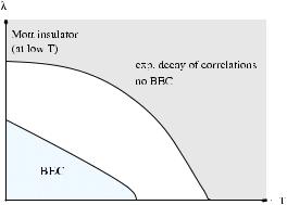
808	M. Aizenman, E.H. Lieb, R. Seiringer, J.P. Solovej and J. Yngvason

2.If either T or λ is big enough, then the one-body density matrix decays exponentially with the distance |x − y|, and hence there is no BEC. In particular, this applies to the ground state T = 0 for λ big enough, where the system is in a Mott insulator phase.

3.The Mott insulator phase is characterized by a gap, i.e., a jump in the chemical potential. We are able to prove this, at half-ﬁlling, in the region described in item 2 above. More precisely, there is a cusp in the dependence of the ground state energy on the number of particles; adding or removing one particle costs a non-zero amount of energy. We also show that there is no such gap whenever there is BEC.

4.The interparticle interaction is essential for items 2 and 3. Non-interacting bosons always display BEC for sufﬁciently low, but positive T (depending on λ, of course).

5.For all T ≥ 0 and all λ > 0 the diagonal part of the one-body density matrix ax†ax (the one-particle density) is not constant. Its value on the A sublattice is constant, but strictly less than its constant value on the B sublattice and this discrepancy survives in the thermodynamic limit. In contrast, in the

regime mentioned in item 1, the off-diagonal long-range order is constant, i.e.,ax†ay ≈ φ (x)φ (y) for large |x − y| with φ (x) = constant.

Fig. 1 Schematic phase diagram at half-ﬁlling

Because of the hard-core interaction between the particles, there is at most one particle at each site and our Hamiltonian (2) thus acts on the Hilbert space H = x Λ C2. The creation and annihilation operators can be represented as 2 × 2 ma-

trices with

ax† ↔	0	1	,	ax ↔	0	0	,	ax†ax ↔	1	0	,
	0	0			1	0			0	0

Quantum Phases of Cold Bosons in an Optical Lattice

809

for each x Λ. More†precisely, these matrices act on the tensor factor associated

with the site x while ax

and ax act as the identity on the other factors in the Hilbert

space H =

x Λ C2.

The Hamiltonian can alternatively be written in terms of the spin 1/2 operators

1 0 1

0 −i

1 0 .

2 1 0

i 0

−

The correspondence with the creation and annihilation operators is

a†

iS2

≡

x =

iS2

≡

−,

x +

x −

and hence ax†ax = Sx3 + 12 . (This is known as the Matsubara-Matsuda correspondence [25].) Adding a convenient constant to make the periodic potential positive, the Hamiltonian (2) is thus equivalent to

= −

+S−

−S+

( 1)xS

x y

+ −

= −

Sx1Sy1 + Sx2Sy2 + λ

+ (−1)xSx3 .

(3)

Without loss of generality we may assume λ ≥ 0. This Hamiltonian is well known as a model for interacting spins, referred to as the XY model [9]. The last term has the interpretation of a staggered magnetic ﬁeld. We note that BEC for the lattice gas is equivalent to off-diagonal long range order for the 1- and 2-components of the spins.

The Hamiltonian (3) is clearly invariant under simultaneous rotations of all the spins around the 3-axis. In particle language this is the U (1) gauge symmetry associated with particle number conservation of the Hamiltonian (2). Off-diagonal long range order (or, equivalently, BEC) implies that this symmetry is spontaneously broken in the state under consideration, cf., e.g. [23]. It is notoriously difﬁcult to prove such symmetry breaking for systems with a continuous symmetry. One of the few available techniques is that of reﬂection positivity (and the closely related property of Gaussian domination) and fortunately it can be applied to our system. For this, however, the hard core and half-ﬁlling conditions are essential because they imply a particle-hole symmetry that is crucial for the proofs to work. Naturally, BEC is expected to occur at other ﬁllings, but no one has so far found a way to prove condensation (or, equivalently, long-range order in an antiferromagnet with continuous symmetry) without using reﬂection positivity and infrared bounds, and these require the additional symmetry.

Reﬂection positivity was ﬁrst formulated by K. Osterwalder and R. Schrader [29, 30] in the context of relativistic quantum ﬁeld theory. Later, J. Fröhlich, B. Simon and T. Spencer used the concept to prove the existence of a phase transition for a classical spin model with a continuous symmetry [16, 15], and E. Lieb and J. Fröhlich [14] as well as F.J. Dyson, E.H. Lieb and B. Simon [9] applied it for the analysis of quantum spin systems. The proof of off-diagonal long range order for

810	M. Aizenman, E.H. Lieb, R. Seiringer, J.P. Solovej and J. Yngvason

the Hamiltonian (3) (for small λ) given here is based on appropriate modiﬁcations of the arguments in [9].

2 Reﬂection Positivity

In the present context reﬂection positivity means the following. We divide the torus Λ into two congruent parts, ΛL and ΛR, by cutting it with a hyperplane orthogonal to one of the d directions. (For this we assume that the side length of Λ is even.) This induces a factorization of the Hilbert space, H = HL HR, with

HL,R =	C2.
	x ΛL,R

There is a natural identiﬁcation between a site x ΛL and its mirror image ϑ x ΛR. If F is an operator on H = HL we deﬁne its reﬂection θ F as an operator on HR in the following way. If F = Fx operates non-trivially only on one site, x ΛL, we deﬁne θ F = V Fϑ xV † where V denotes the unitary particle-hole transformation or, in the spin language, rotation by π around the 1-axis. This deﬁnition extends in an obvious way to products of operators on single sites and then, by linearity, to arbitrary operators on HL. Reﬂection positivity of a state · means that

F θ

≥ 0

(4)

for any F operating on HL. Here F is the complex conjugate of the operator F in the matrix representation deﬁned above, i.e., deﬁned by the basis where the operators

are diagonal.

We now show that reﬂection positivity holds for any thermal equilibrium state of

our Hamiltonian. We can write the Hamiltonian (3) as

S+S−

−S+

(5)

L +

R − 2 xy M

x y +

x y

where HL and HR act non-trivially only on HL and HR, respectively. Here, M denotes the set of bonds going from the left sublattice to the right sublattice. (Because of the periodic boundary condition these include the bonds that connect the right boundary with the left boundary.) Note that HR = θ HL, and

+S−

−S+

+θ S

−θ S

− .

xy M

x y

xy M

For these properties it is essential that we included the unitary particle-hole transformation V in the deﬁnition of the reﬂection θ . For reﬂection positivity it is also important that all operators appearing in H (5) have a real matrix representation. Moreover, the minus sign in (5) is essential.

Quantum Phases of Cold Bosons in an Optical Lattice

811

Using the Trotter product formula, we have

Tr F θ F e−βH = lim Tr F θ F Zn

n→∞

with

e− n1 βHL θ e− n1 βHL

+θ S+

S−θ S

−

. (6)

xy M

x +

Observe that Zn is a sum of terms of the form

Ai θ Ai ,

(7)

with Ai given by either e− n1 βHL or

S+ or

−. All the Ai are real matrices,

and therefore

TrH F θ

Ai θ Ai = TrH F Ai θ

= TrHL F Ai

≥ 0.

(8) Hence Tr F θ F Zn is a sum of non-negative terms and therefore non-negative. This proves our assertion.

3 Proof of BEC for Small λ and T

The main tool in our proof of BEC are infrared bounds. More precisely, for p Λ (the dual lattice of Λ), let Sp# = |Λ|−1/2 x Sx# exp(ip · x) denote the Fourier transform of the spin operators. We claim that

			Sp1, S−1 p	≤	T		(9)
						,
					2Ep	,
with Ep =	d			denotes the components of p, and ( , )
with Ep =	i=1(1 − cos(pi )). Here, pi			denotes the components of p, and ( , )
denotes the Duhamel two point function at temperature T , deﬁned by
			1
	(A, B)	=	Tr Ae−sβH Be−(1−s)βH ds/ Tr e−βH				(10)
		=	0

for any pair of operators A and B. Because of invariance under rotations around the S3 axis, (9) is equally true with S1 replaced by S2, of course.

The crucial lemma (Gaussian domination) is the following. Deﬁne, for a complex valued function h on the bonds xy in Λ,

812			M. Aizenman, E.H. Lieb, R. Seiringer, J.P. Solovej and J. Yngvason
			Z(h) = Tr exp −βK(h) ,					(11)
with K(h) the modiﬁed Hamiltonian
	1			2				2
	1			2				2
K(h) =				Sx+ − Sy− − hxy			+ Sx− − Sy+ − hxy
K(h) =	4	xy		Sx+ − Sy− − hxy			+ Sx− − Sy+ − hxy
		xy		1
	+ λ			1		+ (−1)xSx3 .		(12)

			x		2
			x

Note that for h ≡ 0, K(h) agrees with the Hamiltonian H , because (S±)2 = 0. We claim that, for any real valued h,

Z(h) ≤ Z(0).

(13)

The infrared bound then follows from d2Z(εh)/dε2|ε=0 ≤ 0, taking hxy = exp(ip · x) − exp(ip · y). This is not a real function, though, but the negativity of the (real!) quadratic form d2Z(εh)/dε2|ε=0 for real h implies negativity also for complexvalued h.

The proof of (13) is very similar to the proof of the reﬂection positivity property (4) given above. It follows along the same lines as in [9], but we repeat it here for convenience of the reader.

The intuition behind (13) is the following. First, in maximizing Z(h) one can

restrict to gradients, i.e., hxy =	ˆx −	ˆ y for some function	ˆx on	Λ	. (This fol-
	h	h	h	Λ

lows from stationarity of Z(h) at a maximizer hmax.) Reﬂection positivity implies that Aθ B deﬁnes a scalar product on operators on HL, and hence there is a corresponding Schwarz inequality. Moreover, since reﬂection positivity holds for reﬂections across any hyperplane, one arrives at the so-called chessboard inequality, which is simply a version of Schwarz’s inequality for multiple reﬂections across different hyperplanes. Such a chessboard estimate implies that in order to maximize

h	to be constant. In the case of classical spin
Z(h) it is best to choose the function ˆ x

systems [16, 15], this intuition can be turned into a complete proof of (13). Because of non-commutativity of K(h) with K(0) = H , this is not possible in the quantum case. However, one can proceed by using the Trotter formula as follows.

Let hmax be a function that maximizes Z(h) for real valued h. If there is more than one maximizer, we choose hmax to be one that vanishes on the largest number of bonds. We then have to show that actually hmax ≡ 0. If hmax ≡ 0, we draw a hyperplane such that hxy = 0 for at least one pair xy crossing the plane. We can again write

K(h) = KL(h) + KR (h) +	1		2
K(h) = KL(h) + KR (h) +	4	xy M	Sx+ − Sy− − hxy
		xy M
+ Sx− − Sy+ − hxy	2 .		(14)

Using the Trotter formula, we have Z(h) = limn→∞ αn, with

Quantum Phases of Cold Bosons in an Optical Lattice

αn = Tr e−βKL/ne−βKR /n	e−β(Sx+ −Sy− −hxy)2/4ne−β(Sx− −Sy+ −hxy)2/4n
	xy M
For any matrix, we can write
e−D2 = (4π )−1/2		R dk eikD e−k2/4.

813

(15)

(16)

We apply this to the last two factors Denoting by x1, . . . , xl the points on

in (15), noting that Sy− = θ Sx+ if xy M. the left side of the bonds in M, we then have

αn = (4π )−

R2nl d

2nl

k Tr e−

βK

e−

βK

ik1

−

θ S

+ )β1/2

/2n1/2

. . .

× e−k2/4e−ik1hx1ϑ x1 β1/2/2n1/2....

(17)

Here we denote k2

ki2 for short. Since matrices on the right of M commute

with matrices on the left, and since all matrices in question are real, we see that the trace in the integrand above can be written as

β1/2/2n1/2

e−

βK

ik1S

. . . Tr

e−βKR /ne

θ S

β1/2/2n1/2

(18)

. . . .

Using the Schwarz inequality for the k integration, and ‘undoing’ the above step, we see that

|αn|2 ≤ (4π )−nl

R2nl

d2nl k e−k2/4

× Tr e−

βK

e−

βθ K

ik1(S+

−

θ S

+ )β1/2

/2n1/2

. . .

(4π )−nl

R2nl

d2nl k e−k2/4

× Tr e−

βθ K /n

e−

βK

ik1

(S+

−

θ S+ )β1/2/2n1/2

(19)

. . . .

In terms of the partition function Z(h), this means that

|Z(hmax)|2 ≤ Z(h(1))Z(h(2)),

(20)

where h(1) and h(2) are obtained from hmax by reﬂection across M in the following way:

hxy	if x, y ΛL
hxy(1) = hϑ xϑ y	if x, y ΛR	(21)
0	if xy M

814	M. Aizenman, E.H. Lieb, R. Seiringer, J.P. Solovej and J. Yngvason

and h(2) is given by the same expression, interchanging L and R. Therefore also h(1) and h(2) must be maximizers of Z(h). However, one of them will contain strictly more zeros than hmax, since hmax does not vanish identically for bonds crossing M. This contradicts our assumption that hmax contains the maximal number of zeros among all maximizers of Z(h). Hence hmax ≡ 0 identically. This completes the proof of (13).

The next step is to transfer the upper bound on the Duhamel two point function (9) into an upper bound on the thermal expectation value. This involves convexity arguments and estimations of double commutators like in Sect. 3 in [9]. For this purpose, we have to evaluate the double commutators

	2		1
Sp1	, H, S−1 p + Sp2, [H, S−2 p] = −		H − 2 λ\|Λ\|+2		Sx3Sy3 cos p·(x−y) .
Sp1	, H, S−1 p + Sp2, [H, S−2 p] = −	\|Λ\|	H − 2 λ\|Λ\|+2	xy	Sx3Sy3 cos p·(x−y) .

					(22)
Let Cp denote the expectation value of this last expression,
	Cp = Sp1, H, S−1 p		+ Sp2, H, S−2 p	≥ 0.

The positivity of Cp can be seen from an eigenfunction-expansion of the trace. From [9, Corollary 3.2 and Theorem 3.2] and (9) we infer that

Sp1S−1 p + Sp2S−2 p ≤	1		Cp	coth β2CpEp/4.	(23)
	2		Ep

Using coth x ≤ 1 + 1/x and Schwarz’s inequality, we obtain for the sum over all p = 0,

Sp1S−1 p + Sp2S−2 p ≤	1		1			1		1		1/2	1/2
	1		1		+	1		1			Cp .	(24)

	β	p=	0	Ep		2	p=	0	Ep
p=0		p=	0				p=	0			p=0

We have p Λ Cp = −2 H + λ|Λ|, which can be bounded from above using the following lower bound on the Hamiltonian:

≥ −

|Λ|

d(d

4λ2

1/2

Λ .

(25)

This inequality follows from the fact that the lowest eigenvalue of

−

Syi

−

Syi

λSx

(26)

i=1

is given by − 14 [d(d + 1) + 4λ2]1/2. This can be shown exactly in the same way as [9, Theorem C.1]. Since the Hamiltonian H can be written as a sum of terms like (26), with yi the nearest neighbors of x, we get from this fact the lower bound (25).

With the aid of the sum rule

Quantum Phases of Cold Bosons in an Optical Lattice

815

S1S

|Λ|

−p

p Λ

(which follows from (S1)2

= (S2)2

= 1/4), we obtain from (24) and (25) the

following lower bound in the thermodynamic limit:

Λlim

S01S01 + S02S02

→∞ |

1/2

2 1/2

≥

−

d(d + 1) + 4λ

−

cd ,

(27)

with cd given by

cd =

(28)

(2π )d

[−π,π ]d

This is our ﬁnal result. Note that cd is ﬁnite for d ≥ 3. Hence the right side of (27) is positive, for large enough β, as long as

λ2 < 1 − d(d + 1) . cd2 4

In d = 3, c3 ≈ 0.505 [9], and hence this condition is fulﬁlled for λ 0.960. In [9] it was also shown that dcd is monotone decreasing in d, which implies a similar result for all d > 3.

The connection with BEC is as follows. Since H is real, also γ (x, y) is real and

we have

γ (x, y) = Sx+Sy− = Sx1Sy1 + Sx2Sy2 .

Hence, if ϕ0 = |Λ|−1/2 denotes the constant function,

ϕ0|γ |ϕ0 = S01S01 + S02S02 ,

and thus the bound (27) implies that the largest eigenvalue of γ (x, y) is bounded from below by the right side of (27) times |Λ|. In addition one can show that the infrared bounds imply that there is at most one large eigenvalue (of the order |Λ|), and that the corresponding eigenvector (the ‘condensate wave function’) is strictly constant in the thermodynamic limit [2]. The constancy of the condensate wave function is surprising and is not expected to hold for densities different from 12 , where particle-hole symmetry is absent. In contrast to the condensate wave function the particle density shows the staggering of the periodic potential [2, Theorem 3]. It also contrasts with the situation for zero interparticle interaction, as discussed at the end of this paper.

In the BEC phase there is no gap for adding particles beyond half ﬁlling (in the thermodynamic limit): The ground state energy, Ek , for 12 |Λ| + k particles satisﬁes

0 ≤ Ek − E0 ≤	(const.)			(29)
	\|	Λ	\|

816	M. Aizenman, E.H. Lieb, R. Seiringer, J.P. Solovej and J. Yngvason

(with a constant that depends on k but not on |Λ|.) The proof of (29) is by a variational calculation, with a trial state of the form (S0+)k |0 , where |0 denotes the absolute ground state, i.e., the ground state for half ﬁlling. (This is the unique ground state of the Hamiltonian, as can be shown using reﬂection positivity. See Appendix A in [2].) Also, in the thermodynamic limit, the energy per site for a given density, e( ), satisﬁes

e( ) − e	1	≤ const. −	1	2	(30)
				.
	2		2

Thus there is no cusp at = 1/2. To show this, one takes a trial state of the form

\|ψy = e	iε		S2	1	+	1	\|0 .	(31)
\|ψy = e		x	x	Sy	+	2	\|0 .	(31)
		x	x

The motivation is the following: we take the ground state and ﬁrst project onto a given direction of S1 on some site y. If there is long-range order, this should imply that essentially all the spins point in this direction now. Then we rotate slightly around the S2-axis. The particle number should then go up by ε|Λ|, but the energy only by ε2|Λ|. We refer to [2, Sect. IV] for the details.

The absence of a gap in the case of BEC is not surprising, since a gap is characteristic for a Mott insulator state. We show the occurrence of a gap, for large enough λ, in the next section.

4 Absence of BEC and Mott Insulator Phase

The main results of this section are the following: If either

•λ ≥ 0 and T > d/(2 ln 2), or

•T ≥ 0 and λ ≥ 0 such that λ + |e(λ)| > d, with e(λ) = ground state energy per site,

then there is exponential decay of correlations:

γ (x, y) ≤ (const.) exp(−κ|x − y|)

(32)

with κ > 0. Moreover, for T = 0, the ground state energy in a sector of ﬁxed particle number N = 12 |Λ| + k, denoted by Ek , satisﬁes

Ek + E−k − 2E0 ≥ (λ + |e(λ)| − d)|k|.

(33)

I.e., for large enough λ the chemical potential has a jump at half ﬁlling.

The derivation of these two properties is based on a path integral representation of the equilibrium state at temperature T , and of the ground state which is obtained in the limit T → ∞. The analysis starts from the observation that the density operator e−βH has non-negative matrix elements in the basis in which {Sx3} are diagonal, i.e.

Quantum Phases of Cold Bosons in an Optical Lattice

817

of states with speciﬁed particle occupation numbers. It is convenient to focus on the dynamics of the ‘quasi-particles’ which are deﬁned so that the presence of one at a site x signiﬁes a deviation there from the occupation state which minimizes the potential-energy. Since the Hamiltonian is H = H0 + λW , with H0 the hopping term in (3) and W the staggered ﬁeld, we deﬁne the quasi-particle number operators nx as:

	1	x	3		ax†ax,	for x even
nx =		+ (−1)	Sx	=	1 − ax†ax,	for x odd .	(34)
	2

Thus nx = 1 means presence of a particle if x is on the A sublattice (potential maximum) and absence if x is on the B sublattice (potential minimum).

The collection of the joint eigenstates of the occupation numbers, {|{nx} }, provides a convenient basis for the Hilbert space. The functional integral representation of {nx}| e−β(H0+λW ) |{nx} involves an integral over conﬁgurations of quasiparticle loops in a space × time for which the (imaginary) ‘time’ corresponds to a variable with period β. The fact that the integral is over a positive measure facilitates the applicability of statistical-mechanics intuition and tools. One ﬁnds that the quasi-particles are suppressed by the potential energy, but favored by the entropy, which enters this picture due to the presence of the hopping term in H . At large λ, the potential suppression causes localization: long ‘quasi-particle’ loops are rare, and the amplitude for long paths decays exponentially in the distance, both for paths which may occur spontaneously and for paths whose presence is forced through the insertion of sources, i.e., particle creation and annihilation operators. Localization is also caused by high temperature, since the requirement of periodicity implies that at any site which participates in a loop there should be at least two jumps during the short ‘time’ interval [0, β) and the amplitude for even a single jump is small, of order β.

The path integral described above is obtained through the Dyson expansion
et (A+B) = et A m 0 0≤t1≤t2≤···≤tm≤t B(tm) · · · B(t1)dt1 · · · dtm	(35)
≥

for any matrices A and B and t > 0, with B(t ) = e−t ABet A. (The m = 0 term in

the sum is interpreted here as 1.)

In evaluating the matrix elements of e−βH = e−β(H0+λW ), in the basis {|{nx} }, we note that W is diagonal and {nx}|H0|{nx} is non-zero only if the conﬁgurations {nx} and {nx} differ at exactly one nearest neighbor pair of sites where the change corresponds to either a creation of a pair of quasi-particles or the annihilation of such a pair. I.e., the matrix elements are zero unless nx = nx for all x except for a nearest neighbor pair xy , where nx = ny, nx = ny, and nx + nx = 1. In this case, the matrix element equals −1/2.

Introducing intermediate states, the partition function can thus be written as follows:

818

M. Aizenman, E.H. Lieb, R. Seiringer, J.P. Solovej and J. Yngvason

Tr e−βH =

∞

0≤t1≤t2

≤···≤tm≤β

nx(i)

m=0

}

,1 i

≤

× exp

−λ

(ti − ti−1)

nx(i) dt1 · · · dtm

i=1

× (−1)m {nx(1)}|H0|{nx(m)} {nx(m)}|H0|{nx(m−1)}

× {nx(m−1)}|H0|{nx(m−2)} · · · {nx(2)}|H0||{nx(1)}

(36)

with the interpretation t

lines of (36)

− β. Note that the factor in the last two (i)

} differ by

equals (1/2)m if adjacent elements in the sequence of conﬁgurations {nx

exactly one quasi-particle pair, otherwise it is zero.

Expansions of this type are explained more fully in [1]. A compact way of writing

(36) is:
Tr e−βH = v(dω)e−λ\|ω\|.	(37)

Here the ‘path’ ω stands for a set of disjoint oriented loops in the ‘space-time’ Λ × [0, β], with periodic boundary conditions in ‘time’. Each ω is parametrized by a number of jumps, m, jumping times 0 ≤ t1 ≤ t2 ≤ · · · ≤ tm ≤ β, and a sequence of conﬁgurations {n(i)x }, which is determined by the initial conﬁguration {n(x1)} plus a sequence of ‘rungs’ connecting nearest neighbor sites, depicting the creation or annihilation of a pair of neighboring quasi-particles (see Fig. 2). As in Feynman’s picture of QED, it is convenient to regard such an event as a jump of the quasi-particle, at which its time-orientation is also reversed. The length of ω, denoted by |ω|, is the sum of the vertical lengths of the loops. The measure v(dω) is determined by (36); namely, for a given sequence of conﬁgurations {n(i)x },

1 ≤ i ≤ m, the integration takes places over the times of the jumps, with a measure

(1/2)mdt1 · · · dtm.

One may note that the measure v(dω) corresponds to a Poisson process of random conﬁgurations of oriented ‘rungs’, linking neighboring sites at random times, and signifying either the creation or the annihilation of a pair of quasiparticles. The matrix element {nx}|e−βH |{nx} gets no contribution from rung conﬁgurations that are inconsistent, either internally or with the boundary conditions corresponding to the speciﬁed state vectors. A consistent conﬁguration yields a family of nonoverlapping loops which describe the motion of the quasi-particles in the ‘spacetime’ Λ × [0, β). Each such conﬁguration contributes with weight e−λ|ω| to the above matrix element (another positive factor was absorbed in the measure v(dω)). One may note that long paths are suppressed in the integral (39) at a rate which increases with λ.

Likewise, for x = y, we can write
Tr a†aye−βH	=	v(dω)e−λ\|ω\|,	(38)
x	=	A (x,y)

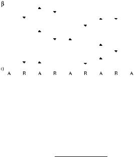
Quantum Phases of Cold Bosons in an Optical Lattice									819

Fig. 2 Loop gas describing paths of quasi-particles for particle number N = |Λ|/2 − 1. A line on an A site means presence of a particle, while on a B site it means absence. The horizontal rungs correspond to hopping of a particle

where A (x,y) denotes the set of all loops that, besides disjoint closed loops, contain one curve which avoids all the loops and connects x and y at time zero. The oneparticle density matrix can thus be written

γ (x, y) =	A (x,y) v(dω)e−λ\|ω\|	(39)
	v(dω)e−λ\|ω\| .

For an upper bound, we can drop the condition in the numerator that the loops and the curve from x to y do not intersect. The resulting measure space is simply a Cartesian product of the measure space appearing in the denominator and the space of all curves, ζ , connecting x and y, both at time 0. Denoting the latter by B(x, y), we thus get the upper bound

γ (x, y) ≤	v(dζ )e−λ\|ζ \|.	(40)
	B(x,y)

The integral over paths is convergent if either λ or T is small enough, and away from the convergence threshold the resulting amplitude decays exponentially. A natural random walk estimate, see [2, Lemma 4], leads to the claimed exponential bound provided

d 1 − e−βλ < λ.

(41)

This includes, in particular, the cases T > d for any λ, and λ > d for any T . Exponential decay actually holds for the larger range of parameters where

d 1 − e−β(λ−f ) < λ − f,

(42)

where f = f (β, λ) = −(β|Λ|)−1 ln Tr e−βH is the free energy per site. Note that f < 0. This condition can be obtained by a more elaborate estimate than the one used in obtaining (40) from (39), as shown in [2, Lemma 3]. The argument there uses reﬂection positivity of the measure v(dω). Using simple bounds on f one can then obtain from (42) the conditions stated in the beginning of this section.

+ λ(−1)x.

820 M. Aizenman, E.H. Lieb, R. Seiringer, J.P. Solovej and J. Yngvason

The proof of the energy gap is based on an estimate for the ratio Tr Pk e−βH where

Tr P0e−βH

Pk projects onto states in Fock space with particle number N = 12 |Λ| + k, expressing numerator and denominator in terms of path integrals. The integral for the numerator is over conﬁgurations ω with a non-trivial winding number k. Each such conﬁguration includes a collection of ‘non-contractible’ loops with total length at least β|k|. An estimate of the relative weight of such loops yields the bound

	Tr Pk e−βH			k
			(const.)( Λ / k )\|k\|	e1−(const.)β \| \|	(43)
	Tr P0e−βH ≤		(const.)( Λ / k )\|k\|	e1−(const.)β \| \|	(43)
	Tr P0e−βH ≤		\| \| \| \|
which gives for β → ∞
		Ek − E0 ≥ (const.)\|k\|			(44)

independently of |Λ|. We refer to [2] for details.

5 The Non-interacting Gas

The interparticle interaction is essential for the existence of a Mott insulator phase for large λ. In case of absence of the hard-core interaction, there is BEC for any density and any λ at low enough temperature (for d ≥ 3). To see this, we have to calculate the spectrum of the one-particle Hamiltonian − 12 + V (x), where denotes the discrete Laplacian and V (x) = λ(−1)x. The spectrum can be easily obtained by noting that V anti-commutes with the off-diagonal part of the Laplacian, i.e., {V , + 2d} = 0. Hence

− d + V (x)

+ λ2,

−

= −

− d

(45)

so the spectrum is given by

d ±

cos pi

+ λ2,

(46)

| |

where p

Λ . In particular, E(p)

−

E(0)

λ2)−1/2

1 d(d2

for small p

and hence there is BEC for low enough temperature. Note that the condensate wave function is of course not constant in this case, but rather given by the eigenfunction corresponding to the lowest eigenvalue of − 12

Quantum Phases of Cold Bosons in an Optical Lattice

821

6 Conclusion

In this paper a lattice model is studied, which is similar to the usual Bose-Hubbard model and which describes the transition between Bose-Einstein condensation and a Mott insulator state as the strength λ of an optical lattice potential is increased. While the model is not soluble in the usual sense, it is possible to prove rigorously all the essential features that are observed experimentally. These include the existence of BEC for small λ and its suppression for large λ, which is a localization phenomenon depending heavily on the fact that the Bose particles interact with each other. The Mott insulator regime is characterized by a gap in the chemical potential, which does not exist in the BEC phase and for which the interaction is also essential. It is possible to derive bounds on the critical λ as a function of temperature.

References

1.M. Aizenman and B. Nachtergaele, Geometric aspects of quantum spin states. Commun. Math. Phys. 164, 17–63 (1994)

2.M. Aizenman, E.H. Lieb, R. Seiringer, J.P. Solovej, and J. Yngvason, Bose-Einstein quantum phase transition in an optical lattice model. Phys. Rev. A 70, 023612-1–12 (2004)

3.O. Alon, A.I. Streltsov, and L.S. Cederbaum, Zoo of quantum phases and excitations of cold bosonic atoms in optical lattices. Phys. Rev. Lett. 95, 030405 (2005)

4.I. Bloch, Exploring quantum matter with ultracold atoms in optical lattices. J. Phys. B 38, S629–S643 (2005)

5.I. Bloch, J. Dalibard, and W. Zwerger, Many-body physics with ultracold gases. Rev. Mod. Phys. 80, 885 (2008)

6.P. Buonsante and A. Vezzani, Phase diagram for ultracold bosons in optical lattices and superlattices. Phys. Rev. A 70, 033608 (2004)

7.E. Calzetta, B.L. Hu, and A.M. Rey, Bose–Einstein condensate superﬂuid-Mott insulator transition in an optical lattice. Phys. Rev. A 73, 023610 (2006)

8.D.B.M. Dickerscheid, D. van Oosten, P.J.H. Denteneer, and H.T.C. Stoof, Ultracold atoms in optical lattices. Phys. Rev. A 68, 043623 (2003)

9.F.J. Dyson, E.H. Lieb, and B. Simon, Phase transitions in quantum spin systems with isotropic and nonisotropic interactions. J. Stat. Phys. 18, 335–383 (1978)

10.N. Elstner and H. Monien, Dynamics and thermodynamics of the Bose-Hubbard model. Phys. Rev. B 59, 12184–12187 (1999)

11.R. Fernándes, J. Fröhlich, and D. Ueltschi, Mott transition in lattice boson models. Commun. Math. Phys. 266, 777–795 (2006)

12.M.P.A. Fisher, P.B. Weichman, G. Grinstein, and D.S. Fisher, Boson localization and the superﬂuid-insulator transition. Phys. Rev. B 40, 546–570 (1989)

13.J.K. Freericks and H. Monien, Strong-coupling expansions for the pure and disordered BoseHubbard model. Phys. Rev. B 53, 2691–2700 (1996)

14.J. Fröhlich and E.H. Lieb, Phase transitions in anisotropic lattice spin systems. Commun. Math. Phys. 60, 233–267 (1978)

15.J. Fröhlich, B. Simon, and T. Spencer, Infrared bounds, phase transitions and continuous symmetry breaking. Commun. Math. Phys. 50, 79 (1976)

16.J. Fröhlich, B. Simon, and T. Spencer, Phase transitions and continuous symmetry breaking.

Phys. Rev. Lett. 36, 804 (1976)

822	M. Aizenman, E.H. Lieb, R. Seiringer, J.P. Solovej and J. Yngvason

17.J.J. Garcia-Ripoll, J.I. Cirac, P. Zoller, C. Kollath, U. Schollwoeck, and J. von Delft, Variational ansatz for the superﬂuid Mott-insulator transition in optical lattices. Opt. Express 12, 42–54 (2004)

18.M. Greiner, O. Mandel, T. Esslinger, T.E. Hänsch, and I. Bloch, Quantum phase transition from a superﬂuid to a Mott insulator in a gas of ultracold atoms. Nature 415, 39 (2002)

19.M. Greiner, O. Mandel, T.E. Hänsch, and I. Bloch, Collapse and revival of the matter wave ﬁeld of a Bose-Einstein condensate. Nature 419, 51 (2002)

20.D. Jaksch and P. Zoller, The cold atom Hubbard toolbox. Ann. Phys. (N.Y.) 315, 52–79 (2005)

21.D. Jaksch, C. Bruder, J.I. Cirac, C.W. Gardiner, and P. Zoller, Cold bosonic atoms in optical lattices. Phys. Rev. Lett. 81, 3108–3111 (1998)

22.T. Kennedy, E.H. Lieb, and S. Shastry, The XY model has long-range order for all spins and all dimensions greater than one. Phys. Rev. Lett. 61, 2582–2584 (1988)

23.E.H. Lieb, R. Seiringer, and J. Yngvason, Bose-Einstein condensation and spontaneous symmetry breaking. Rep. Math. Phys. 59, 389–399 (2007)

24.M.M. Maska, R. Lemanski, J.K. Freericks, and C.J. Williams, Pattern formation in mixtures of ultracold atoms in optical lattices. Phys. Rev. Lett. 101, 060404 (2008)

25.T. Matsubara and H. Matsuda, A lattice model of liquid helium. Progr. Theor. Phys. 16, 569– 582 (1956)

26.O. Morsch and M.K. Oberthaler, Dynamics of Bose-Einstein condensates in optical lattices. Rev. Mod. Phys. 78, 179–215 (2006)

27.Ch. Moseley, O. Fialko, and K. Ziegler, Interacting bosons in an optical lattice. Ann. Phys. (Berlin) 17, 48 (2008)

28.Z. Nazario and D.I. Santiago, Quantum states of matter of simple bosonic systems: BEC’s, superﬂuids and quantum solids. Phys. Lett. A 328, 207–211 (2004)

29.K. Osterwalder and R. Schrader, Axioms for Euclidean Green’s functions. Commun. Math. Phys. 31, 83–112 (1973)

30.K. Osterwalder and R. Schrader, Commun. Math. Phys. 42, 281–305 (1975)

31.V.G. Rousseau and P.J.H. Denteneer, Quantum phases of mixtures of atoms and molecules on optical lattices. Phys. Rev. A 77, 013609 (2008)

32.S. Sachdev, Quantum Phase Transitions. Cambridge University Press, Cambridge (1999)

33.V.W. Scarola and S. Das Sarma, Quantum phases of the extended Bose-Hubbard Hamiltonian: Possibility of a supersolid state of cold atoms in optical lattices. Phys. Rev. Lett. 95, 033003 (2005)

34.R. Schmied, T. Roscilde, V. Murg, D. Porras, and J.I. Cirac, Quantum phases of trapped ions in an optical lattice. New J. Phys. 10, 045017–045035 (2008)

35.D. van Oosten, P. van der Straten, and H.T.C. Stoof, Quantum phases in an optical lattice. Phys. Rev. A 63, 053601 (2001)

36.K. Ziegler, Phase transition of a Bose gas in an optical lattice. Laser Phys. 13, 587–593 (2003)

37.W. Zwerger, Mott-Hubbard transition of cold atoms in optical lattices. J. Opt. B 5, 9–16 (2003)

<<< < Предыдущая 37 38 39 40 41 42 43 44 45 46 47 4849 / 6849 50 51 52 53 54 55 56 57 58 59 60 61 > Следующая >>>

Соседние файлы в папке Diss

#
27.03.20161.6 Mб5127.pdf
#
27.03.20167.05 Mб17228.pdf
#
27.03.20161.31 Mб523.pdf
#
27.03.2016838.41 Кб484.pdf
#
27.03.2016451.11 Кб425.pdf
#
27.03.201615.34 Mб486 - 753p.pdf
#
27.03.2016451.11 Кб406.pdf
#
27.03.2016499.39 Кб457.pdf
#
27.03.20161.47 Mб438.pdf
#
27.03.201615.42 Кб41Введение.docx
#
27.03.201619.78 Кб43Список литературы.docx