Diss / 8

Abstract—In this paper, we propose a maximum-entropy expec- tation-maximization (MEEM) algorithm. We use the proposed algorithm for density estimation. The maximum-entropy constraint is imposed for smoothness of the estimated density function. The derivation of the MEEM algorithm requires determination of the covariance matrix in the framework of the maximum-entropy likelihood function, which is difficult to solve analytically. We, therefore, derive the MEEM algorithm by optimizing a lower-bound of the maximum-entropy likelihood function. We note that the classical expectation-maximization (EM) algorithm has been employed previously for 2-D density estimation. We propose to extend the use of the classical EM algorithm for image recovery from randomly sampled data and sensor field estimation from randomly scattered sensor networks. We further propose to use our approach in density estimation, image recovery and sensor field estimation. Computer simulation experiments are used to demonstrate the superior performance of the proposed MEEM algorithm in comparison to existing methods.

Index Terms—Expectation-maximization (EM), Gaussian mixture model (GMM), image reconstrution, Kernel density estimation, maximum entropy, Parzen density, sensor field estimation.

I. INTRODUCTION

STIMATING an unknown probability density function E(pdf) given a finite set of observations is an important aspect of many image processing problems. The Parzen windows method [1] is one of the most popular methods which provides a nonparametric approximation of the pdf based on the underlying observations. It can be shown to converge to an arbitrary density function as the number of samples increases. The sample requirement, however, is extremely high and grows dramatically as the complexity of the underlying density function increases. Reducing the computational cost of the Parzen windows density estimation method is an active area of research. Girolami and He [2] present an excellent review of recent developments in the literature. There are three broad categories of methods adopted to reduce the computational cost of the Parzen windows density estimation for large sample sizes: a) approximate kernel decomposition method [3], b) data

Manuscript received March 29, 2007; revised January 13, 2008. The associate editor coordinating the review of this manuscript and approving it for publication was Dr. Gaurav Sharma.

The authors are with the Multimedia Communications Laboratory, Department of Electrical and Computer Engineering, University of Illinois at Chicago, Chicago, IL 60607-7053 USA (e-mail: hhong6@uic.edu; dans@uic.edu).

Color versions of one or more of the figures in this paper are available online at http://ieeexplore.ieee.org.

Digital Object Identifier 10.1109/TIP.2008.921996

reduction methods [4], and c) sparse functional approximation method.

Sparse functional approximation methods like support vector machines (SVM) [5], obtain a sparse representation in approximation coefficients and, therefore, reduce computational costs for performance on a test set. Excellent results are obtained using these methods. However, these methods scale as making them expensive computationally. The reduced set density estimator (RSDE) developed by Girolami and He [2] provides a superior sparse functional approximation method which is designed to minimize an integrated squared-error (ISE) cost function. The RSDE formulates a quadratic programming problem and solves it for a reduced set of nonzero coefficients to arrive at an estimate of the pdf. Despite the computational efficiency of the RDSE in density estimation, it can be shown that this method suffers from some important limitations [6]. In particular, not only does the linear term in the ISE measure result in a sparse representation, but its optimization leads to assigning all the weights to zero with the exception of the sample point closest to the mode as observed in [2] and [6]. As a result, the ISE-based approach to density estimation degenerates to a trivial solution characterized by an impulse coefficient distribution resulting in a single kernel density function as the number of data samples increases.

However, the expectation-maximization algorithm (EM) [7] provides a very effective and popular alternative for estimating model parameters. It provides an iterative solution, which converges to a local maximum of the likelihood function. Although the solution to the EM algorithm provides the maximum likelihood estimate of the kernel model for density function, the resulting estimate is not guaranteed to be smooth and may still preserve some of the sharpness of the ISE-based density estimation methods. A common method used in regularization theory to ensure smooth estimates is to impose the maximum entropy constraint. There have been some attempts to bind the entropy criterion with EM algorithm. Byrne [8] proposed an iterative image reconstruction algorithm based on cross-entropy minimization using the Kullback–Leibler (KL) divergence measure [9]. Benavent et al. [10] presented an entropy-based EM algorithm for the Gaussian mixture model in order to determine the optimal number of centers. However, despite the efforts to use maximum entropy to obtain smoother density estimates, thus far, there have been no successful attempts to expand the EM algorithm by incorporating a maximum-entropy penalty-based approach to estimating the optimal weight, mean and covariance matrix.

In this paper, we introduce several novel methods for smooth kernel density estimation by relying on a maximum-entropy

penalty and use the proposed methods for the solution of important applications in image reconstruction and sensor field estimation. The remainder of the paper is organizes as follows. In Section II, we first introduce kernel density estimation and present the integrated squared-error (ISE) cost function. We subsequently introduce the maximum-entropy ISE-based density estimation to ensure that the estimated density function is smooth and does not suffer from the degeneracy of the ISE-based kernel density estimation. Determination of the maximum-entropy ISE-based cost function is a difficult task and generally requires the use of iterative optimization techniques. We propose the hierarchical maximum entropy kernel density estimation (HMEKDE) method by using a hierarchical tree structure for the decomposition of the density estimation problem under the maximum-entropy constraint at multiple resolutions. We derive a closed-form solution to the hierarchical maximum-entropy kernel density estimate for implementation on binary trees. We also propose an iterative solution to a penalty-based maximum-entropy density estimation by using Newton’s method. The methods discussed in this section provide the optimal weights for kernel density estimates which rely on fixed kernels located at few samples. In Section III, we propose the maximum-entropy expectation maximization (MEEM) algorithm to provide the optimal estimates of the weight, mean, and covariance for kernel density estimation. We investigate the performance of the proposed MEEM algorithm for 2-D density estimation and provide computer simulation experiments comparing the various methods presented for the solution of maximum-entropy kernel density estimation in Section IV. We propose the application of both the EM and MEEM algorithms for image reconstruction from randomly sampled images and sensor field estimation from randomly scattered sensors in Section V. The basic EM algorithm estimates a complete data set from partial data sets, and, therefore, we propose to use the EM and MEEM algorithms in these image reconstruction and sensor network applications. We present computer simulations of the performance of the various methods for kernel density estimation for these applications and discuss the advantages and disadvantages in various applications. A discussion of the performance of the MEEM algorithm as the number of kernels varies is provided in Section VI. Finally, in Section VII, we provide a brief summary and discussion of our results.

II.KERNEL-BASED DENSITY ESTIMATION

A. Parzen Density Estimation

The parzen density estimator using the Gaussian Kernel is given by Torkkola [11]

(1)

where is the total number of observation and is the isotropic Gaussian kernel defined by

The main limitation of the Parzen windows density estimator is the very high computational cost due to the very large number of kernels required for its representation.

B. Kernel Density Estimation

We seek an approximation to the true density of the form

(3)

where and the function denotes the Gaussian kernel defined in (2). The weights must be determined such that the overall model remains a pdf, i.e.,

(4)

Later in this paper, we will explore the simultaneous optimization of the mean, variance, and weights of the Gaussian kernels. Here, we focus exclusively on the weights . The variances and means of the Gaussian kernels are estimated by using the -means algorithm in order to reduce the computational burden. Specifically, the centers of the kernels in (3) are determined by -means clustering, and the variance of the kernels is set to the mean of Euclidean distance between centers [12]. We assume that is significantly greater than since the Parzen method relies on delta functions at the sample data which are represented by Gaussian functions with very narrow variance. The mixture of Gaussian model, on the other hand, relies on a few Gaussian kernels and the variance of each Gaussian function is designed to capture many sample points.

Therefore, only the coefficients are unknown. We rely on minimization of the error between and using the ISE method. The ISE cost function is given by

(5)

Substituting and , using (1) and (3), the equation can be expanded and the order of integration and summation exchanged. Thus, we can write the cost function of (5) in vectormatrix form

(6)

where

(7)

is positive semi-definite [13]. Therefore, can be simplified to

.

In Appendix A, we prove that the solution of the ISE-based kernel density estimation degenerates as the number of observations increases to a trivial solution that concentrates the estimated probability mass in a single kernel. This degeneracy leads to a sharp peak in the estimated density, which is characterized by the minimum-entropy solution.

C. Maximum-Entropy Kernel Density Estimation

Given observations from an unknown probability distribution, there may exist an infinity of probability distributions consistent with the observations and any given constraints [14]. The maximum entropy principle states that under such circumstances we are required to be maximally uncertain about what we do not know, which corresponds to selecting the density with the highest entropy among all candidate solutions to the problem. In order to avoid degenerate solutions to (6), we maximize the entropy and minimize the divergence between the estimated distribution and the Parzen windows density estimate. Here, we use Renyi’s quadratic entropy measure given by [11], which is defined as

Newton’s method for multiple variables is given in [15]

(12)

where denotes the iteration. We will use the soft-max function for the weight constraint [16]. The weight of the center can be expressed as

(13)

Therefore, the derivative of the weight with respect to is given by

(14)

.

For convenience, we define the following variables:

(15)

(16)

Since the logarithm is a monotonic function, maximizing the logarithm of a function is equivalent to maximizing the function. Thus, the maximum entropy solution of the entropy can be reached by maximizing the function expressed in vector-matrix form

The derivation of the gradient is provided in Appendix B. From (57), (58), and (62), the element of the Hessian matrix is given by the following.

a)

(10)

where is subject to the constraints provided by (4).

1) Penalty-Based Approach Using Newton’s Method: We adopt the penalty-based approach by introducing an arbitrary constant to balance between the ISE and entropy cost functions. We, therefore, define a new cost function given by

where is the penalty coefficient. Since the variable is constant with respect to it will be omitted. We now have

(11)

(21)

b)

(22)

The detailed derivation of the Hessian matrix are also presented in Appendix B. We assume that the Hessian matrix is positive definite. Finally, the gradient and Hessian required for the iteration in (12) can be generated using (21), (22), and (59).

2) Constrained-Based Approach Using a Hierarchical Binary Tree: Our preference is to avoid penalty-based methods and to derive the optimal weights as a constrained optimization problem. Specifically, we seek the maximum entropy weights

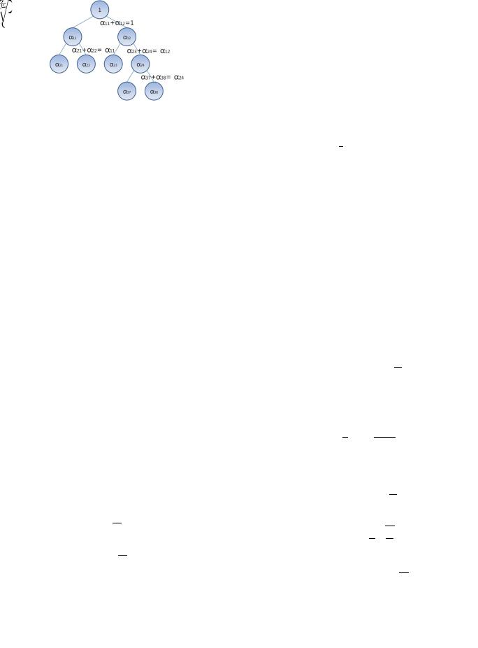
Fig. 1. Binary tree structure for hierarchical density estimation.

The constraint in the maximum entropy problem is defined such that its corresponding ISE cost function does not exceed the optimal ISE cost beyond a prespecified value . From (6), (25), and (26), we can determine the optimal ISE coefficient by minimization of the cost given by

(27)

such that . It is easy to show that

A closed-form solution to this problem is difficult to obtain in general. However, we can obtain the closed-form solution when the number of centers is limited to two. Hence, we form an iterative process, where we assume that we only have two centers at each iteration. We represent this iterative process as a hierarchical model, which generates new centers at each iteration. We use a binary tree to illustrate the hierarchical model, where each node in the tree depicts a single kernel. Therefore, in the binary tree, each parent node has two children nodes as seen in Fig. 1. The final density function corresponds to the kernels at the leafs of the tree. We now wish to determine the maximum entropy kernel density estimation at each iteration of the hierarchical binary tree. We, therefore, seek the maximum entropy coefficients. Note that sum of these coefficients is dictated by the corresponding coefficients of their parent node. This restriction will ensure that the sum of the coefficients of all the leave nodes (i.e., nodes with no children) is one since we set the coefficient of the root parent node to 1. We simplify the notation

method at each node. Let us adopt the following notation:

(24)

(28)

Therefore, from (6), (25), (26), and (28), we have

From (10) and (25), we observe that the maximum entropy

.

Therefore, from (30), we form the Lagrangian given by

Differentiating with respect to and setting to zero, we have

(31)

We shall now determine the Lagrange multiplier by satisfying the constraint

(32)

From (31) and (32), we observe that

(33)

Therefore, from (33) and (31), we observe that

III. MAXIMUM-ENTROPY

EXPECTATION-MAXIMIZATION ALGORITHM

As seen in previous section, the ISE-based methods enable pdf estimation given a set of observations without information about the underlying density. However, the ISE based solutions do not fully utilize the sample information as the number of samples increases. Moreover, ISE-based methods are generally used to determine optimal weights used in the linear combination. Selection of the mean and variance of the kernel functions is accomplished by using the -means algorithm, which can be viewed as a hard limiting case of the EM [7]. The EM algorithm offers an approximation of the pdf by an iterative optimization under the maximum likelihood criterion.

A probability density function can be approximated as the sum of Gaussian functions

(35)

where is center of a Gaussian function, is a covariance matrix of function and is the weight for each center which subject to the conditions as (4). The Gaussian function is given by

The expectation step of the EM algorithm can be separated into two terms, one is the expectation related with likelihood and the other is the expectation related with the entropy penalty

(40)

(41)

where denotes that this expectation is from the likelihood function, denotes that this expectation is from the entropy penalty, and denotes the number of iteration.

The Jensen’s inequality is applied to find the new lower bound of the likelihood functions using (40) and (41). Therefore, the lower bound function for the likelihood function can be derived as

(36)

From (35) and (36), we observe that the logarithm of the likelihood function for the given Gaussian mixture parameters that has observations can be written as

(37)

where is the sample and is a set of parameters (i.e., the weights, centers, and covariances) to be estimated.

The entropy term is added in order to make the estimated density function smooth and not to have an impulse distribution. We expand Renyi’s quadratic entropy measure [11] to incorporate with covariance matrices and use the measure again. Substituting (35) into (8), expanding the square and interchanging the order of summation and integration, we obtain the following:

(38)

We, therefore, form an augmented likelihood function parameterized by a positive scalar in order to simultaneously maximize the entropy and likelihood using (37) and (38). The augmented likelihood function is given by

bound, we, therefore, rely on a monotonically decreasing and concave function such that . The detailed derivation is provided in Appendix C. Notice that maximization of the entropy remains unchanged if we replace the function in (38) by since both are monotonically decreasing functions. We can now use Jensens inequality to obtain the lower bound for the entropy

A. Mean

The new estimates for the mean vectors can be obtained by the derivative of (43) with respect to and setting it to zero. Therefore

(44)

(47)

Using (47) and the symmetric property of Gaussian, we thus introduce a new lower bound for the covariance given by

B. Weight

For the weights, we once again use the soft-max function in (13) and (14). Thus, by setting the derivative of with respect to to zero, the new estimated weight is given by

(45)

C. Covariance

In order to update the EM algorithm, the derivative of (43) with respect to is required. However, the derivative cannot be solved directly because of the existence of the inverse matrix which appears in the derivative. We, therefore, introduce a new lower bound for the EM algorithm using Cauchy–Schwartz inequality. The lower bound given by (43) can be rewritten as

inequality and the fact that the Gaussian function is greater than or equal to zero, we obtain

We note that the EM algorithm presented here relies on a simple extension of the lower-bound maximization method in [17]. In particular, we can use this method to prove that our algorithm converges to a local maximum on the bound generated by the Cauchy–Schwartz inequality, which serves as a lower bound on the augmented likelihood function. Moreover, we would have attained a local maximum of the augmented likelihood function had we not used the Cauchy–Schwartz inequality to obtain a lower bound for the sum of the covariances. Note that the Cauchy–Schwartz inequality is met with equality if and only if the covariance matrices of the different kernels are identical. Therefore, if the kernels are restricted to have the same covariance structure, the maximum-entropy expecta- tion-maximization algorithm converges to a local maximum of the augmented likelihood function.

IV. TWO-DIMENSIONAL DENSITY ESTIMATION

We apply MEEM method and other conventional methods to a 2-D density estimation problem. Fig. 2(a) describes original 2-D density function and Fig. 2(b) displays a scatter plot of 500 data samples drawn from (49) in the interval [0,1]. The equation used for generating the samples is given by

(49)

where . Given data without knowledge of the underlying density function used to generate the observations, we must estimate the 2-D density function. Here, we use 500, 1000, 1500, and 2000 samples for the experiment. With the exception of the RSDE method, the other approaches cannot be used to determine the optimal number of centers since it will

fluctuate based on variations in the problem (e.g., initial conditions). We determine the number of centers experimentally such that we assign less than 100 samples per center for Newton’s method, EM and MEEM. For the HMEKDE method, we terminate the splitting of the hierarchical tree when the leaf has less than 5% of total number of samples.

The results of RSDE are shown in Fig. 2(c). RSDE method is very powerful algorithm in that it requires no parameters for the estimation. However, the choice for the kernel width is very crucial since it suffers the degeneracy problem when the kernel width is large and the reduction performance is diminished when the kernel width is small. The results of Newton’s method and HMEKDE are given in Fig. 2(d) and (e), respectively. The major practical issue in implementing Newton’s method is the guarantee of local minimum, which can be sustained by positive definitiveness of Hessian matrix [15]. Thus, we use the Levenberg–Marquardt algorithm [18], [19]. The value in HMEKDE method is chosen experimentally. The results of the conventional EM algorithm and the MEEM algorithm are shown in Fig. 2(f) and (g), respectively. The variable in MEEM algorithm is chosen experimentally. The result of MEEM is properly smoothed.

In Fig. 3, SNR improvements according to iteration and the value of is displayed using 300 samples. We choose the value as proportional to the number of samples. The parameter values multiplied by the number of samples, are shown in Fig. 3 (i.e., 0.05, 0.10, and 0.15). We observe the over-fitting problem of the EM algorithm in Fig. 3. The overall improvements in SNR are given in Table I.

V. IMAGE RECONSTRUCTION AND SENSOR FIELD ESTIMATION

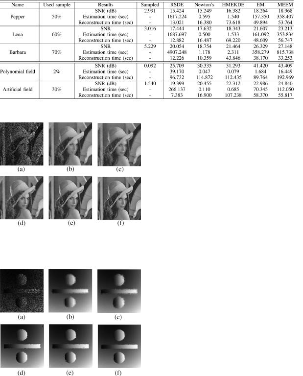
Density estimation problem can easily expanded into practical problems like image reconstruction from random sample. For experiment, we use 256 256 gray Pepper, Lena, and Barbara images which is shown in Fig. 4(a)–(c).

We take 50% samples of Pepper image, 60% samples of Lena image and 70% of Barbara image. We use density function model in [20] where is the intensity value and

is the location of a pixel. We estimate a density function of given image from samples. For the reduction of computational

Fig. 4. Three 256 2 256 gray images used for the experiments. (a) Pepper,

(b) Lena, and (c) Barbara and two sensor fields used for sensor field estimation from randomly scattered sensor: (d) polynomial sensor field and (e) artificial sensor field.

burden, 50% overlapped 16 16 blocks are used for the experiment. Since the smoothness is different from block to block, we choose the smoothing parameter for each block experimentally. The initial center location is equally spaced. We use 3 3 centers for experiment. Using the estimated density function, we can estimate the intensity value of given location using expectation operation of conditional density distribution function. The sampled image and the reconstruction results of Lena are shown in Fig. 5.

We can also expand our approach into the estimation of sensor field from randomly scattered sensors. In this experiment, we generate an arbitrary field using polynomials in Fig. 4(d) and an artificial field in Fig.4(e). The original sensor field is randomly sampled and 2% of samples is used for the polynomial field and 30% of samples are used for the artificial field. We use density function model where L is intensity value and is the location of sensor. 50% overlapped 32 32 blocks and 16

16 blocks are used for the estimation of polynomial sensor field and artificial sensor field respectively for computational time. We also choose the smoothing parameter for each block experimentally. The initial center location is equally spaced. We use 3 3 centers for each experiment. We estimate a density function of given field using sensors. For each algorithm except HMEKDE, we use equally spaced centers for the initial location of center. The sampled sensor field and the estimation results of

Fig. 5. Comparison of density estimation for image reconstruction from randomly sampled image. (a) 60% sampled image; (b) RSDE; (c) HMEKDE;

(d) Newton’s method; (e) conventional EM; (f) MEEM.

In this section, we discuss the relationship between the number of center and minimum/maximum entropy. Our experimental results indicate that, in most cases, the results under the maximum entropy show better results than the conventional EM algorithm. However, in some limited cases, like when we use a small number of centers, the results of minimum entropy penalty shows better results than the results of the conventional EM algorithm and maximum entropy penalty. This is due to the characteristics of maximum and minimum entropy, which is well described in [21]. The maximum entropy solution provides us smooth solution. In the case that the number of centers are relatively sufficient, each center can represent piecewise one Gaussian component, which means the resulting density function can be described better under maximum entropy criterion. On the contrary, the minimum entropy solution gives us the least smooth distribution. In the case that the number of centers are insufficient, each center should represent a large number of samples; thus, the resulting distribution described by a center should be the least smooth one, since each center cannot be described in terms of piecewise Gaussian any more. However, the larger number of centers used, the better the result.

Fig. 6. Comparison of density estimation for artificial sensor field estimation from randomly scattered sensor. (a) 30% sampled sensor; (b) RSDE;

(c) HMEKDE; (d) Newton’s method; (e) conventional EM; (f) MEEM.

artificial field are given in Fig. 6. The signal to noise ratio of the results and the computational time are also given in Table II.

VII. CONCLUSION

In this paper, we develop a new algorithm for density estimation using the EM algorithm with a ME constraint. The proposed MEEM algorithm provides a recursive method to compute a smooth estimate of the maximum likelihood estimate. The MEEM algorithm is particularly suitable for tasks that require the estimation of a smooth function from limited or partial data, such as image reconstruction and sensor field estimation. We demonstrated the superior performance of the proposed MEEM algorithm in comparison to various methods (including the traditional EM algorithm) in application to 2-D density estimation, image reconstruction from randomly sampled data, and sensor field estimation from scattered sensor networks.

(54)

Taking logarithms on both sides and multiplying by 1, we

(59), we observe that

This completes the proofs. From the proposition above, we observe that the ISE-based kernel density estimation yields the lowest entropy kernel density estimation. It results in a kernel density estimate that consists of a single kernel. This result presents a clear indication of

the limitation of ISE-based cost functions.

APPENDIX B

GRADIENT AND HESSIAN IN NEWTON’S METHOD

In this appendix, we provide the detailed derivation of the gradient and the Hessian matrix of (12). First, we present the

(58)

Thus, the element of the gradient can be expressed as

(59)

The element of the Hessian matrix can be expressed as

a)

(60)

b)

(61)