

Diss / 7
.pdfProceedings of the International MultiConference of Engineers and Computer Scientists 2008 Vol II IMECS 2008, 19-21 March, 2008, Hong Kong
Direction of Arrival Estimation using a Root-MUSIC Algorithm
H. K. Hwang, Zekeriya Aliyazicioglu, Marshall Grice, Anatoly Yakovlev
Abstract—An array antenna system with innovative signal processing can enhance the resolution of a signal direction of arrival (DOA) estimation. Super resolution algorithms take advantage of array antenna structures to better process the incoming signals. They also have the ability to identify multiple targets. This paper explores the eigen-analysis category of super resolution algorithm. A class of Multiple Signal Classification (MUSIC) algorithms known as a root-MUSIC algorithm is presented in this paper.
The root-MUSIC method is based on the eigenvectors of the sensor array correlation matrix. It obtains the signal estimation by examining the roots of the spectrum polynomial. The peaks in the spectrum space correspond to the roots of the polynomial lying close to the unit circle.
Statistical analysis of the performance of the processing algorithm and processing resource requirements are discussed in this paper. Extensive computer simulations are used to show the performance of the algorithms.
Index Terms— Array antenna, Direction of arrival estimation, Signal processing.
I. INTRODUCTION
Accurate estimation of a signal direction of arrival (DOA) has received considerable attention in communication and radar systems of commercial and military applications. Radar, sonar, and mobile communication are a few examples of the many possible applications. For example, in defense application, it is important to identify the direction of a possible threat. One example of commercial application is to identify the direction of a emergency cell phone call such that the rescue team can be dispatched to the proper location.
DOA estimation using a fixed antenna has many limitations. Its resolution is limited by the antenna’s mainlobe beamwidth. Antenna mainlobe beamwidth is inversely proportional to its physical size. Improving the accuracy of angle measurement by increasing the physical aperture of the receiving antenna is not always a practical
This work was supported in part by the Raytheon
H. K. Hwang and Zekeriya Aliyazicioglu are with the Electrical and Computer Engineering Department, California State Polytechnic University, Pomona, CA 91768 USA, (e-mail: hkhwang@ csupomona.edu and zaliyazici@csupomona.edu).
Marshall Grice was a graduate student at California State Polytechnic University, Pomona, CA. He is now with the Boeing, CA. (e-mail: grice@csupomona.edu)
Anatoly Yakovlev was an undergraduate student at California State Polytechnic University, Pomona, CA. He is now with Western Digital, San Jose, CA 95138, USA (e-mail: Anatoly.Yakovlev@wdc.com)
option. Certain systems such as a missile seeker or aircraft antenna have physical size limitations; therefore they have relatively wide mainlobe beamwidth. Consequently, the resolution is quite poor. Also, if there are multiple signals falling in the antenna mainlobe, it is difficult to distinguish between them.
Instead of using a single antenna, an array antenna system with innovative signal processing can enhance the resolution of signal DOA. An array sensor system has multiple sensors distributed in space. This array configuration provides spatial samplings of the received waveform. A sensor array has better performance than the single sensor in signal reception and parameter estimation. Its superior spatial resolution provides a means to estimate the direction of arrival (DOA) of multiple signals. A sensor array also has applications in interference rejection [1], electronic steering [2], multi-beam forming [3], etc. This technology is now widely used in communications, radar, sonar, seismology, radio astronomy ,etc.
There are many different super resolution algorithms including spectral estimation, model based, and eigen-analysis to name a few [4,5,6]. In this paper, we concentrate the discussion on the application of estimating the DOA of multiple signals. The focuses are on a class of Multiple Signal Classification (MUSIC) algorithms known as root-MUSIC and an extension of root-MUSIC. We present detailed MATLAB simulation results for each algorithm.
II. ARRAY SENSOR SYSTEMS
We use an array antenna with a 16 element uniform linear array (ULA) in this paper. Fig. 1 shows the general configuration for a ULA antenna having M elements arranged along a straight line with the distance between sensor elements, be d = λ/2, where λ is the incoming signal wavelength. The angle of the incoming signal, θ, is measured relative to the antenna bore sight.
Bore sight
|
|
Incoming |
|
|
|
θ |
Signal |
|
|
|
|
|
|
|
|
|
|
d= λ/2 |
|
1 |
2 |
3 |
4 |
M |
|
|
|
|
Sensor Elements |
Figure 1. ULA Antenna configuration
ISBN: 978-988-17012-1-3 |
IMECS 2008 |
Proceedings of the International MultiConference of Engineers and Computer Scientists 2008 Vol II IMECS 2008, 19-21 March, 2008, Hong Kong
For the a conventional antenna, the main lobe beam width (MLBW) of an antenna manner is given by, in radians
MLBW = k |
λ |
(1) |
|
D |
|||
|
|
where D is the diameter of the antenna array and k is a proportionality constant, for most case k ≈1 [6].
III. ROOT-MUSIC ALGORITHM
The root-MUSIC method relies on the following properties of the array correlation matrix: the space spanned by its eigenvectors may be partitioned into two orthogonal subspaces, namely the signal plus noise subspace and the noise only subspace; the steering vectors corresponding to the directional sources are orthogonal to the noise subspace [7]. The MxM correlation matrix that contains L number of incoming signals is formed by
R = SDSH +σ2I |
(2) |
where σ2 is the variance of the Gaussian white noise, D is the signal power matrix and S is the signal direction matrix
D = diag[P1, P2,...PL]
|
1 |
1 |
|
e− jβ(θ1) |
e− jβ(θ2) |
S = |
... |
... |
|
||
e− j(M −1)β(θ1) |
e− j(M −1)β(θ2) |
|
|
|
|
(3) |
... |
|
1 |
|
... |
e |
− jβ(θL) |
|
... |
|
||
... |
|
|
|
... |
|
|
|
e− j(M −1)β(θL) |
|||
subspace and the remaining M-L eigenvectors will span the noise only subspace, QN. By eigen-analysis we can represent the M-L smallest eigenvectors as
Rq |
i |
=σ2q |
i |
i = L +1,..., M |
. |
(7) |
|
|
|
|
|
||||
Using (7) in (2), can be rewritten as |
|
|
|||||
SDSHqi |
= 0 |
i = L +1,..., M |
|
(8) |
|||
Since S is a full column rank matrix and D is diagonal, (8)
becomes |
|
|
SHqi = 0 |
i = L +1,..., M |
(9) |
or more explicitly |
|
|
sk Hqi = 0 |
i = L +1,..., M |
. |
(10) |
|
k =1,..., L |
||
|
|
|
Equation (10) proves the orthogonality between the signal plus noise and the noise only subspaces. This is important because it shows that the angle of the incoming signals can be found by searching for signal direction vectors that, when projected onto the noise only subspace, give a zero result. Following this idea, if a polynomial, J(z), is constructed such that
J (z) = vHQNQNH v = 0 |
(11) |
where the steering vector v is
and the phase delay between sensor elements is |
|
(4) |
|
|
|
|
|
|
|
|
|
|
|
|
T |
||||||||
|
|
v = 1 |
z |
−1 |
z |
−2 |
z |
−( M −1) |
|
||||||||||||||
(4) |
|
|
|
|
|
|
|
|
|
|
|
|
|
(12) |
|||||||||
|
β(θi) = |
2πd |
sin(θi) |
|
|
(5) |
|
|
|
|
|
|
|
|
|
|
|
|
|
||||
|
|
|
|
and |
|
|
|
|
|
|
|
|
|
|
|
|
|||||||
|
|
|
|
|
|
|
|
|
|
|
|
|
|
|
|
|
|||||||
|
|
|
|
λ |
|
|
|
|
|
|
|
|
|
|
|
|
|
|
|
|
|
|
|
Let |
λ ≥ λ ≥... ≥ λ |
be the |
eigenvalues |
of |
the |
z = e |
j |
2πd |
sin(θ) |
|
|
|
|
|
|
||||||||
λ |
|
|
|
|
|
|
|
||||||||||||||||
|
1 |
2 |
|
M |
|
|
|
|
|
|
|
|
|
|
|
. |
|
|
|
|
(13) |
||
correlation matrix R, and |
υ1 ≥υ2 ≥... ≥υL |
be |
the |
|
|
|
|
|
|
|
|
|
|
||||||||||
Then the roots of J(z) contain the directional information |
|||||||||||||||||||||||
eigenvalues for SDSH . Then from (2) |
|
|
|||||||||||||||||||||
|
|
|
|
|
|
|
|
|
|
of the incoming signals. Ideally, the roots of J(z) would be on |
|||||||||||||
|
|
|
2 |
i |
=1, 2,...L |
|
|
the unit circle at locations determined by the directions of the |
|||||||||||||||
|
λi |
|
(6) |
incoming signals; however, due to the presence of noise the |
|||||||||||||||||||
|
= υi +σ |
|
|
||||||||||||||||||||
|
|
σ2 |
|
i = L +1,...M |
|
|
roots may not necessarily be on the unit circle. In this case, |
||||||||||||||||
|
|
|
|
|
|
|
|
|
|
the L closest roots to the unit circle are the roots that |
|||||||||||||
For |
high |
signal to |
noise |
ratios |
(SNR) υi σ2 . The |
correspond to the L incoming signals [9]. These selected |
|||||||||||||||||
eigenvalues can be used to determine the number of sources |
roots, by themselves, do not directly represent the incoming |
||||||||||||||||||||||
angle. For each root, the incoming angle is found by solving |
|||||||||||||||||||||||
that are detected by counting the number of comparatively |
(13). |
|
|
|
|
|
|
|
|
|
|
|
|
||||||||||
large eigenvalues. Alternatively, Ref. [7] suggests a more |
|
|
|
|
|
|
|
|
|
|
|
|
|
||||||||||
rigorous approach to determining the number of incoming |
|
|
|
|
|
|
λ |
|
|
|
|
|
|
||||||||||
|
|
|
|
|
|
|
|
|
|
|
|
|
|
|
|
|
|
|
|
||||
sources that provides better detection performance when the |
θk = arcsin |
|
|
|
arg(zk ) |
|
|
|
|||||||||||||||
2πd |
|
|
|
||||||||||||||||||||
incoming SNR is not as high. For the purposes of this, the |
|
|
|
|
|
|
|
. |
|
(14) |
|||||||||||||
incoming SNR is chosen to be sufficiently high as to not be in |
Obviously, when the root-MUSIC algorithm is |
||||||||||||||||||||||
a situation where the source number detection is ambiguous. |
|||||||||||||||||||||||
implemented there is no prior knowledge of the incoming |
|||||||||||||||||||||||
Let q1, q2, … , qM be the eigenvectors associated with the |
|||||||||||||||||||||||
signal directions or signal powers needed to construct the |
|||||||||||||||||||||||
decreasing ordered eigenvalues λ1 ≥ λ2 ≥... ≥ λM . From |
|||||||||||||||||||||||
correlation matrix using (2). Therefore the correlation matrix |
|||||||||||||||||||||||
(6) the first L eigenvectors will span the signal plus noise
ISBN: 978-988-17012-1-3 |
IMECS 2008 |

Proceedings of the International MultiConference of Engineers and Computer Scientists 2008 Vol II IMECS 2008, 19-21 March, 2008, Hong Kong
must be estimated using only the information available from |
β(θi ) = |
2π(d +ei ) |
sin(θi ) |
|
|||||||
the sensor array. There are several methods commonly used |
|
||||||||||
|
(17) |
||||||||||
to perform this estimation such as temporal averaging, spatial |
|
λ |
|||||||||
|
|
|
|
||||||||
smoothing or, a hybrid combination of both temporal |
|
When these data are applied to the root-MUSIC algorithm, |
|||||||||
averaging and spatial smoothing [8]. In this paper, we use |
|||||||||||
(14) no longer has the correct value for d and obviously will |
|||||||||||
only the temporal averaging method. |
|
|
|
||||||||
|
|
|
return a result that has some increased error. |
|
|||||||
|
|
|
|
|
|
|
|
||||
The estimated correlation matrix using the temporal |
|
|
|
|
|
||||||
averaging method with k snapshots is given as |
|
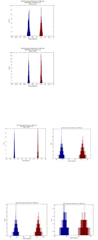
B. Root-Music Simulation Results |
|
||||||||
Φ = E[AH A] |
|
|
|
|
|
Statistical results, Fig.4 , show that two incoming signals |
|||||
|
|
|
|
(15) |
are clearly identified even as the separation between the two |
||||||
where the incoming data matrix A is |
|
|
|
signals is well below the conventional main lobe beam width. |
|||||||
|
|
|
It can be seen that as the spacing between signals decreases |
||||||||
|
|
|
|
|
|
|
the variance of the estimates increases. The average |
||||
u (1) |
u (2) ... |
u (k) |
|
|
|
estimation error is in all cases nearly zero. |
|
||||
1 |
1 |
|
1 |
|
|
|
|
|
|
|
|
A = u2 (1) |
u2 (2) ... |
u2 (k) |
|
|
|
|
|
1 Beam Width Separation: |
|||
|
|
|
|
|
|
|
|
|
|||
... |
... |
... |
... |
|
|
|
|
|
Average Estimated Angle = |
||
uM (1) |
uM (2) ... |
uM (k) |
. |
(16) |
39.9972 |
46.0041 |
|||||
|
|
|
|
|
|
|
Average Estimation Error= |
||||
with ui(k) being the ith sensor output at time k. |
|
0.0028 |
-0.0041 |
||||||||
|
|
|
Mean Square Error = |
||||||||
The estimated correlation matrix, Φ, asymptotically |
|
0.0009 |
0.0012 |
||||||||
|
|
|
|
|
|||||||
approaches the correlation matrix, R as the number of |
|
|
|
|
|
||||||
snapshots increases. Therefore in order to have an accurate |
|
|
|
|
|||||||
estimation of the correlation matrix the observation time must |
|
(a) |
|
||||||||
be sufficiently long. The long observation times are not ideal |
|
|
|||||||||
for radar signal processing applications; however there are |
|
|
1/2 Beam Width Separation: |
||||||||
many applications where this does not pose a problem. |
|
|
|
||||||||
Correlation matrix estimation techniques like the spatial |
|
|
Average Estimated Angle = |
||||||||
39.9988 |
42.9995 |
||||||||||
smoothing method are better suited for use in time sensitive |
|||||||||||
|
|
Average Estimation Error= |
|||||||||
systems. |
|
|
|
|
|
|
0.0012 |
0.0005 |
|||
|
|
|
|
|
|
|
|
|
Mean Square Error = |
||
|
|
|
|
|
|
|
0.0023 |
0.0025 |
|||
A. Sensor Spacing and Phase Sensitivity
The root-MUSIC algorithm assumes that each sensor is perfectly spaced relative to the other sensors in the array. While this holds true for the theoretical case, perfect sensor spacing is difficult to achieve when the algorithm is actually implemented even with modern construction techniques. The method by which the algorithm is modified to model these variations is rather straight forward. The sensor spacing problem is characterized by Fig.3.
(b)
1/4 Beam Width Separation:
Average Estimated Angle =
39.9999 41.4987
Average Estimation Error=
0.0001 0.0013
Mean Square Error =
0.0047 0.0042
Incoming
Signal
|
θ |
|
d+e3 |
d+e4 |
|
|
d+e1 |
|
d+e2 |
d+eM |
|||
|
d= |
λ/2 |
||||
|
|
|||||
|
|
|
|
|
||
1 |
2 |
|
3 |
4 |
|
M |
|
Variation in Distance |
|
|
Ideal Sensor |
||
|
between Sensor Elements |
|
Elements |
|||
Figure 3. Non-ideal ULA sensor spacing
The spacing error of each sensor, ei, is a Gaussian random variable added to the ideal spacing. Taking this error into account, (5) is used to create the phase shift between sensor elements for the incoming signals becomes
(c)
Figure 4. Statistical comparison for 2 signals at various separation angles
Fig.5 shows the effect of increasing the number of snap shots used for the temporal averaging correlation matrix estimation. The estimation variance decreases with increased observation times. The average estimation error does not seem to be very sensitive to the observation time
ISBN: 978-988-17012-1-3 |
IMECS 2008 |
Proceedings of the International MultiConference of Engineers and Computer Scientists 2008 Vol II IMECS 2008, 19-21 March, 2008, Hong Kong
1/4 Beam Width Separation
32 Snap Shots:
Average Estimated Angle =
39.9999 41.4987
Average Estimation Error=
0.0001 0.0013
Mean Square Error =
0.0047 0.0042
(a)
1/4 Beam Width Separation
96 Snap Shots:
Average Estimated Angle =
39.9992 41.5008
Average Estimation Error=
0.0008 -0.0008
Mean Square Error =
0.0015 0.0016
(b)
Figure 5. Variation of snap shot comparison
In Fig.6, We compare the simulation results of ideally spaced sensor elements against the results of a simulation where the sensor elements have a 1% random variance in their spacing; in other words σ = λ / 200 .
The algorithm does exhibit a rather strong sensitivity to the positional accuracy of the sensor placement; however with proper array calibration these effects could be minimized.
IV. CONCLUSION
We have presented the root-MUSIC method based on the eigenvector of the sensor array correlation matrix to estimate angle of incoming signals. We give extensive computer simulation results to demonstrate the performance of the algorithms, which enhance the DOA estimation.
The simulation results of the root-MUSIC algorithm show the following results
1.The capability to resolve multiple targets with separation angles smaller the main lobe beam width of the array antenna.
2.The estimation variance can be reduced by increasing the number of snapshots in correlation matrix estimation
3.The estimation variance increases as the angle separation between signals becomes smaller
4.The estimation variance depends on the direction of the signal. A signal coming from the bore sight has minimum estimation variance.
ACKNOWLEDGMENT
Figure 6. Comparison of Non-Ideal Sensor Spacing
Increasing the amount of spacing variance from 1% to 5% shows an increased error variance in Fig.7. It is worth noting that while the performance of the algorithm decreases with increased sensor spacing error the algorithm is still able to successfully distinguish both incoming signal directions.
Figure 7. MUSIC Spectrum with Two Signals from (65°, 15°) and (65°, 25°)
The simulation results of the root-MUSIC algorithm clearly demonstrate the ability to resolve multiple targets with separation angles smaller then the main lobe beam width of the array thus proving its super-resolution capabilities.
The authors would like to thank the Raytheon Corporation for its support of this investigation.
REFERENCES
[1].Anne Lee, Lijia Chen, H. K. Hwang and et al. “Simulation Study of Wideband Interference Rejection using Adaptive Array Antenna”. IEEE Aerospace Conference, March 5-12, 2005
[2].M. G. M. Hussain, Performance Analysis and Advancement of Self-Steering Arrays for Nonsinusoidal Waves, IEEE Trans. on Electromagnetic Compatibility, May 1988
[3].X. Zhang and D. Su, Digital Processing System for Digital Beam Forming Antenna, IEEE International Symposium on Microwave, Antenna Propagation and EMC Technologies, 2005
[4].Jianmin Zhu, Megan Chan and H. K. Hwang, “Simulation Study on Adaptive Antenna Array” IEEE International Signal Processing Conference, Dallas, 2003
[5].Marshall Grice, Jeff Rodenkirch, Anatoly Yakovlev, H. K. Hwang, Z. Aliyazicioglu, Anne Lee, “Direction of Arrival Estimation using Advanced Signal Processing”, RAST Conference , Istanbul-Turkey, 2007.
[6].Skolnik, Merrill. Introduction to RADAR Systems. 3rd ed. New York: Mc Graw Hill, 2001.
[7].Godara, Lal Chand, Smart Antennas. Boca Raton: CRC Press, 2004
[8].Kuo, Chen Yu. Wideband Signal Processing for Super Resolution DOA Estimation. Pomona: California State Polytechnic University Pomona, 2006.
[9].Forsythe, Keith. “Utilizing Waveform Features for Adaptive Beamforming and Direction Finding with Narrowband Signals.” Lincoln Laboratory Journal 10.2 (1997): 99-126.
ISBN: 978-988-17012-1-3 |
IMECS 2008 |